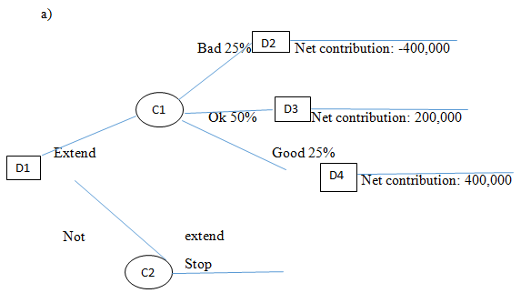
AbFab has a higher probability of accruing profits when the credit is extended. Only a probability of 0.25 will lead to losses. The remaining 0.75 guarantees AbFab to get profits.   From the decision tree diagram, AbFab should offer credit to S&M (Barry de Ville, 2013).

1. In this case we will do a sensitivity analysis. This will involve analysing how values of independent variable ‘manufacturer’ affect AbFab’s choice of extending credit (Valentine Fontama, 2014). For manufacturer A, the risk category “Good” has a probability of 50%, “OK” has a probability of 30% and “Bad” 10%. From this we realize that credit rating A guarantees a high probability of 80% of getting value for money after offering credit services to them. Credit rating B gives actual risk category “bad” a 40% probability. This is close to half meaning that “good” and “OK” isk categories has 60% probability. Credit rating C, the risk category “bad” has a 50% impact on its selection. Since the main objective of AbFab is to recover the funds credited to other companies, they should use actual risk category “Good” to evaluate their potential customers. The probability of the actual risk category “Good” should have the highest value. For “Bad”, the probability must be at the minimum level as much as possible.
2. We create a graph to analyse each actual risk category.

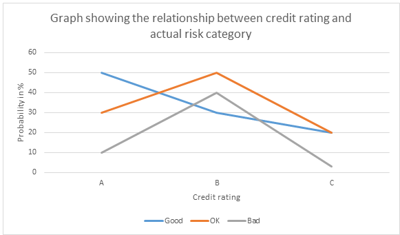
 From the graph we see the variations in probability from one credit rating to another. This shows that in depth analysis is required to ascertain each category. With less resources, the variations will not be clearly defined and laid out. The results can be malicious in instances where the agency lacked enough financial base to deeply scrutinize the manufacturer. The amount of money paid to agencies plays a big role in achieving the desired results. Poorly paid agencies will not conduct proper research and analysis of the data to obtain the optimal course of action. Shoddy research and analysis bring about undesirable results.

• From the graph in c, the largest probability obtained is 50%. In some instances, probability can be as high as 90% which is approximately double what was achieved in our case. In order to optimize the ratings, the agency require more resources in terms of finance. Thus to obtain detailed and accurate results the agency require double the funds initially given to them. From 30,000 pounds, the amount should be doubled to 60,000 pounds.
• First we note that there are two types of predictive models; classification models and regression models. Classification predicts class membership whereas regression models predicts a number. These two models are composed of algorithms. These algorithms are run to execute data mining and analysis of data, projecting trends and patterns depicted by the data. Decision tree is one of the predictive models used. It is created by algorithms that splits the data keyed into the machine to form branch-like segments. It partitions the data into subsets according to the types of input variables. The output produced assists in finding path of decisions.

Part 2 Oxymoron

1. Initially there were three employees who were among them one was to be fired. In terms of probability, each one had a one-third chance of being laid off and two-third chance of remaining (Marshall, 2011). When one employee is cleared and will continue with the job, the number of employees facing risk of firing reduces to two people. Among the two, only one will be laid off. This means that there is 50% survival which is equivalent to a probability of 0.16. Similarly, classic Monty Hall describes how removal of one item increases the probability of the remaining items (Moscovich, 2011). In this case, when there were three employees, the probability of one of them being laid off was . When one employee was removed from the list, the probability increased to . Therefore Theresa was right.
2.  In instances where unequal probabilities exists between the employees, each employee will have different probability of being fired. The person with the highest probability will have the highest chance of being laid off. Since Theresa has the lowest probability of leaving the job.

References

Barry de Ville, P. N., 2013. Decision Trees for Analytics Using SAS Enterprise Miner. In: s.l.:SAS Institute, pp. 42-67.

Marshall, J., 2011. The Math Dude’s Quick and Dirty Guide to Algebra. In: Quick & Dirty Tips. s.l.:St. Martin’s Press, pp. 133-157.

Moscovich, I., 2011. The Monty Hall Problem and Other Puzzles. In: Dover Recreational Math Series. s.l.:Dover Publications, pp. 33-47.

Valentine Fontama, R. B. W. H. T., 2014. Predictive Analytics with Microsoft Azure Machine Learning: Build and Deploy Actionable Solutions in Minutes. In: s.l.:Apress, pp. 4-15.