Introduction

There are many cases where the relation of motion can be shown with respect to time. Spring mass system is an example of harmonic motion. It follows Hook’s law and Newton’s law of motion. Displacement, velocity, and acceleration can be found of any motion by the help of those laws. In order to get the solution, we need to solve differential equations. In this study, we will discuss various methods of solving differential equations. Analytical, Euler, ODE45, numerical methods are used in this study for solving the governing equation of spring damping system. Matlab helps us in solving any equation correctly and also in a quick process. The processes, codes, and methods are required in performing a Matlab program. This study will help in deriving and solving the governing equation for the spring-mass-damping system and also will help to analyze the key findings during solving by the use of Matlab.

Question 1

a)

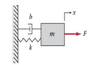
Fig 1: Spring mass damping system

(Source: http://ctms.engin.umich.edu/CTMS/index.php?example=Introduction&section=SystemModeling)

(i) Governing equation describes about the change of unknown variables with change of known ones. There is governing equations related to different motions. In case of this spring, a mass of m is held there by MSD. Force F is applied on it for oscillating purpose (Harris, 2017). Force of the damper is given, where b is damping constant. Spring constant k is given there. Deriving a governing equation, below steps can be used:

F= ma;

a= dx²/dt²;

Considering gravity force, spring force and damping force in this:

mg – k(s+x) = F – b * dx/dt;

mg – k(s+x) = mdx²/dt² – b * dx/dt;

This is the governing equation for the given figure.

(ii) The conditions here are given for the figure where the governing equation is needed to be solved. The conditions provided are;

F= 0, m=10 kg, k= 160N/ m, b= 0 N s/m;

x(0) = 0, dx/dt |_x=0 = 6;

Gravity force is taken here as negligible. So, force due to gravity is eliminated in the equation. Besides, spring force is also taken as zero for ease in solution (Cárcamo, Gómez & Fortuny, 2016).

mdx²/dt² + kx= 0;

dx²/dt² + (k/m)x = 0;

dx²/dt² + (160/10)x = 0;

dx²/dt² + 16x = 0;

Taking the ODE for solution:

D²+ 16= 0;

D= ± 4;           

Appendix 1: Symbolic form of solution in Matlab

x(t) = c₁ cost 4t + c₂ sin 4t;                                         

As, x(0) = 0;

0 = c₁ cost 0 + c₂ sin 0 =  c₁ ;

So, x(t) =  c₂ sin 4t;

x’(t) = 4c₂ cos 4t;

As, dx/dt |_x=0 = 6, 4c₂ = 6

c₂ = 3/2= 1.5;

So, x(t) = 1.5 sin 4t;

This is the solution for governing equation in this case.

(iii) By the help of Matlab symbolic software it is noted that above solution is correct. The command history regarding that is shown below: [Referred to Appendix 1]

syms x t;
dsolve(‘D2y+16*y=0’)
syms x t;
dsolve(‘D2x+16*x=0’, ‘Dx(0)=6’, ‘x(0)=0’, ‘t’)

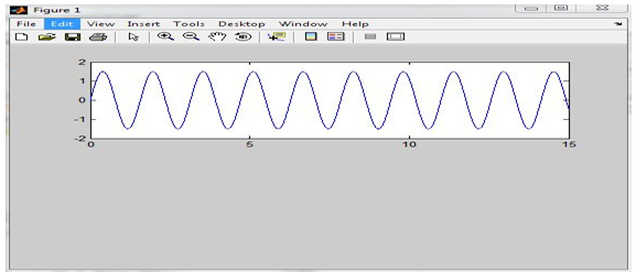
(iv) Plotting of curves with respect to displacement and time is done in Matlab using below codes: [Referred to Appendix 2]

Appendix 2: Displacement graph

clear all;

>> close all;

>> t= 0:0.01:15;

>> x= 1.5*sin(4*t);

>> subplot(2,1,1);

>> plot(t,x);

(v) Adding the damping function will provide different result in this case. Damping coefficient is taken as 4N s/m. This gives a different solution in this case (Chen et al. 2017). The solution given in this case is done by the help of Matlab by code:

syms x t;

dsolve(‘D2x-4Dx+16*x=0’, ‘Dx(0)=6’, ‘x(0)=0’, ‘t’)

This gives the solution as:

x= 3/2*sin(4t)-1/4*cos(4t)+¼;

This makes a change in displacement as can be seen in displacement by plotting curve:

clear all;

close all;

t= 0:0.01:3;

x= 1.5*sin(4*t)-0.25*cos(4*t)+0.25;

clear all;

t= 0:0.01:15;

x= 3/2*sin(4*t)-1/4*cos(4*t)+1/4;

subplot (2,1,1);

plot(t,x); [Refferred to Appendix 3]

Appendix 3: Damping factor in solution

(b)

Euler’s method coding is done to plot the curves in Matlab. Codes used are:

clear all;

close all;

clc;

f=@(t,y)t+y;

t0=0;

y0=6;

h=0.001;

tn=1;

n=(tn-t0)/h;

T(1)=t(0);

Y(1)=y(0);

for i=2:n

    Y(i)= Y(i-1)+ h*feval(f,T(i-1),Y(i-1));

    T(i)=T(i-1)+h;

end

figure(1);

sol=dsolve(‘Dy=t+y’,’y(0)=6′, ‘t’);

y_exact= inline(vectorize(sol));

plot(T,y_exact(T),’b*-‘);

xlabel(‘t’);

ylable(‘y(t)’);

hold on;

plot (T, Y, ‘ro-‘);

legend(‘Exact Solution’, ‘Approx. Solution’) [Refferred to Appendix 4]

Appendix 4: Euler’s method solution

Different time steps are used in this method. The time steps given in the jobs are 0.1, 0.002, I have taken another time step 0.001 to better result. Before doing this second order equation in two 1st order. Then the equations are solved by the help of numerical methods. Different steps are used for different plotting purpose.

(c) Using ODE45 in Matlab for solving the same equation is done which gives a different plot of graph. Codes of that part is:

tspan = [0 5];

y0 = 0;

[t,y] = ode45(@(t,y) 2*t, tspan, y0);

>> plot(t,y,’-o’)

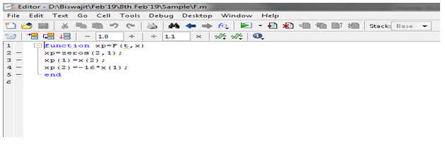
function xp=F(t,x)

xp=zeros(2,1);

xp(1)=x(2);

xp(2)=-16*x(1);

end [Refferred to Appendix 5]

Appendix 5: Function for ODE45

[t,x]=ode45(‘F’,[0,15],[0,6]);

[t,x(:,1)]

plot(t,x(:,1)) [Refferred to Appendix 6]

Appendix 6: Plotting of ODE solution

This is the function for making a proper solution in ODE45 method. 2nd order ODE is solved by this method and the solution is plotted in Matlab.

(d)

(i) Changing of the values of m and k will give different solutions. In cases where spring’s constant is made higher, we find less duration of oscillations. And for another case, if the constant is made lower the duration of oscillation becomes higher. Also for the cases where mass is lighter, it will get shorter period of oscillations (Cook, 2018). This is the changes found when m and k are used as different values in the above equations. Graph’s results changes according to the values.

(ii) The initial conditions are taken as initial displacement -2m and initial velocity 0m/s. This changes the solution of the equation. This is done on Matlab. Codes used in this case will be changed as:

syms x t;

dsolve(‘D2x+16*x=0’, ‘Dx(0)=0’, ‘x(0)=-2’, ‘t’)

And this gives a solution:

Ans, x = -2cos(4t) [Refferred to Appendix 7]

Appendix 7:

Key findings

After doing total analysis of this spring damp system we have come to different conclusion. Those can be discussed as below:

• Governing equation of motion is derived in spring-mass system. It helps to know the changes and relation of spring mass, constant, displacement and other factors. The conditions given here are gravity force as zero and zero friction effect. With the help of this governing equation is made up.
• Solution of governing equation for MSD is made with the help of analytical method first. For that purpose, we need to know some values of variables. The variable’s values have effect on the solution. Displacement is a dependent variable which changes with change of time. The solution we get provides idea about the dependency of displacement on time, which follows sin or cosine graphs.
• Matlab symbolic solver is a useful method to confirm about the solution. The solutions made by analytical method can be rechecked by the help of symbolic solver. “dsolve” is the call function which gives solution.
• By plotting the graphs of those solution shows the displacement of spring mass with respect to time. Time duration of change needs to be done in small displacement which shows a clear image.
• Damping factor in spring are neglected in previous solution which provides a infinite harmonic solution. But implementing damping factor in study will provide a negative force in the motion. Harmonic motion tends to reduce its frequency and amplitude with increment of time and becomes zero after a period of time. This is shown by the graphs with the help of Matlab.
• Euler’s and ODE45 methods are also used for doing the solution. Euler’s method takes lots of step for getting solution in 2nd order ODE. As we have to transform it into 1st order and then make the solution. In this process steps needed are higher in comparison. More steps allow chances of more errors in job. In other hand, ODE45 method is capable of doing up to 4-5th order solutions of ODE. Still, it needs to be reduced to 1st order for implementing in Matlab.
• Effect of mass and spring constant is also there in spring-mass oscillation. As we can see after solving and changing the values of m and k in equations, that the solutions changes with these change. When the mass gets reduced the period will be shorter and vice versa. But in case of spring constant where it gets reduced the period increases (Engelbrecht Bergsten & Kågesten, 2017). This can be seen by applying different values of m and k.
• Changing initial conditions gives different results. Gives different result in solutions and in graphs as well. It gives graphs of cos function. The code changes to:

syms x t;

dsolve(‘D2x+16*x=0’, ‘Dx(0)=0’, ‘x(0)=-2’, ‘t’)

ans =

-2*cos(4*t)

close all;

t= 0:0.01:15;

x= -2*cos(4*t);

subplot(2,1,1);

plot(t,x)

Question 2

a)

>> Mass = 10

k = 160

% Pick zeta, find B

%zeta = .71

%B = zeta*2*sqrt(k*Mass)  % n/(m/sec) damping

% given B and Mass, find zeta

B = 0

zeta = B/(2*sqrt(k*Mass))

omegan = sqrt(k/Mass)  % naturalfreq

K = 1/k  % static gain

sys = tf((omegan^2)/k, [1 2*zeta*omegan omegan^2])

pole(sys)

omegad = omegan*sqrt(1-zeta^2) % damped nat freq

Td = 2*pi/omegad  % damped period

Tp = Td/2       % peak time

ymax = K*(1+exp(-zeta*omegan*Tp))       % peak magnitude [Referred to Appendix 8]

Appendix 8: Spring damper system

T98 = 4/(zeta*omegan)

OmegaPeak = omegan*sqrt(1-2*zeta^2)

MagPeak = K/(2*zeta*sqrt(1-zeta^2))

dBpeak = 20*log10(MagPeak)

PhaseB1 = omegan*(1/5)^zeta

PhseB2 = omegan*5^zeta

figure(1)

PoleLoc = pole(sys);

if isreal(PoleLoc)

    xx = zeros(length(PoleLoc));

    plot( PoleLoc, xx,’*’)

else

    plot(PoleLoc,’*’)

end

grid on

%axis([-2.5 0 -1 1])

axis equal

hold on

title(‘Pole Location’)

xlabel(‘Real Axis’)

ylabel(‘Imaginary axis’)

figure(2)

step(sys)

grid on

hold on

figure(3)

bode(sys)

grid on

hold on

Mass =    10

k =   160

B =     0

zeta =     0

omegan =     4

K =    0.0063

Transfer function:  0.1

——–

s^2 + 16

ans =

        0 + 4.0000i

        0 – 4.0000i

omegad =     4

Td =    1.5708

Tp =    0.7854

ymax =    0.0125

T98 =   Inf

OmegaPeak =     4

MagPeak =   Inf

dBpeak =   Inf

PhaseB1 =     4

PhseB2 =     4 [Referred to Appendix 9]

Appendix 9: spring damper system output

b)

>> m=10; %kg

k=160; %N/m

c=300; %kg/s

vo=-1/1000; %m/s

xo=0.4/1000; %m

t=linspace(0,4,100);

wn=sqrt(k/m) %natural frequency

zeta=c/(2*m*wn) %damping ratio

a1=xo;

a2=vo+wn*xo;

xt=(a1+a2.*t).*(exp(-wn.*t));%general response [Referred to Appendix 10]

Appendix 10: Plot displacement

display(c)

plot(t,xt)

grid on

ylabel(‘x(t)’)

xlabel (‘t’)

wn =    4

zeta =  3.7500

 c =   300

 >>

>> m = 10;  % 1 kg

c = 20; % 12 N-s/m

k = 160; % 20 N/m

% Open-Loop Response

s = tf(‘s’);

P = 1/(m*s^2 + c*s + k) % Transfer function

step(P)

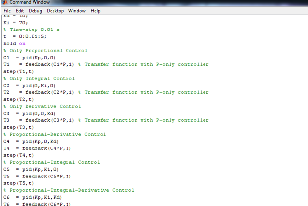
% PID Control Values

Kp = 200;

Kd = 10;

Ki = 70;

% Time-step 0.01 s

t  = 0:0.01:5;

hold on

% Only Proportional Control

C1  = pid(Kp,0,0)

T1   = feedback(C1*P,1) % Transfer function with P-only controller

step(T1,t)

% Only Integral Control

C2  = pid(0,Ki,0)

T2   = feedback(C2*P,1) % Transfer function with P-only controller

step(T2,t)

% Only Derivative Control

C3  = pid(0,0,Kd)

T3   = feedback(C3*P,1) % Transfer function with P-only controller

step(T3,t) [Referred to Appendix 11]

Appendix 11: plot displacement output

c)

function  SMDode_linear(Mass,Damping, Stiffness)

%SMDode_linear.m  Spring-Mass-Damper system behavior analysis for given Mass, Damping and Stiffness values.

%   The system’s damper has linear properties.

%   Solver ode45 is employed; yet, other solvers, viz. ODE15S, ODE23S, ODE23T,

%   ODE23TB, ODE45, ODE113, ODESET, etc., can be used as well.

%   Sulaymon L. ESHKABILOV

%   $Revision: ver. 01 $  $Date: 2011/02/05 02:00:00 $

% Problem parameters, shared with nested functions.

 if nargin < 1

  % ——– Some default values for parameters: Mass, Damping & Stiffness

  % ——– in case not specified by the user

   Mass = 10;       % [kg]

   Damping=50;      % [Nsec^2/m^2]

   Stiffness=200;   % [N/m]  

 end

tspan = [0; max(20,5*(Damping/Mass))]; % Several periods

u0 = [0; 1];                           % Initial conditions

options = odeset(‘Jacobian’,@J);       % Options for ODESETs can be switched off

[t,u] = ode45(@f,tspan,u0,options);

figure;

plot(t,u(:,1),’r*–‘, t, u(:,2), ‘bd:’, ‘MarkerSize’, 2, ‘LineWidth’, 0.5 );

title([‘Spring-Mass-Damper System of 2nd order ODE: ‘, ‘ M = ‘ num2str(Mass),…

   ‘[kg]’ ‘; D = ‘ num2str(Damping), ‘[Nsec^2/m^2]’, ‘; S = ‘ num2str(Stiffness), ‘[N/m]’]);

xlabel(‘time t’);

ylabel(‘Displacement & Velocity’); grid on;

axis tight;

% axis([tspan(1) tspan(end) -1.5 1.5]); % Axis limits can be set  

hold on;  [Referred to Appendix 12]

Fig 2: Gravitational effect on spring

(Source: https://math.la.asu.edu/~milner/coursepages/MAT275/LAB08.pdf)

Appendix 12: Coding on ODE45

The motion of the spring and the mass is being analyzed in this situation. It can be said that when the spring is not loaded with any mass or anything then the then the length of the spring is lo then when the mass is being attached then the length changes to l. Therefore the formula that is derived is:-  mg |{z} downward weight force + −k(` − `0) | {z } upward tension force = 0. The term g that has been used is gravitational acceleration. (g ‘ 9.8m/s2 ‘ 32f t/s2 ). [Referred to Appendix 13]

Appendix 13: Output when the variations are changed as per exertion of force

The unit k is used to measure the effectiveness of the stiffness of the spring on a constant basis. Then when the mass is being pulled by a mass then the formula tends to be mg |{z} weight + −k(` + y − `0) | {z } upward tension force = m d 2 (` + y) dt2 | {z } acceleration of mass , i.e., m d 2y dt2 + ky = 0.This is ODE second order. d 2y dt2 + ω 2 0 y = 0

Where ω 2 0 = k/m. Equation (L8.3) models simple harmonic motion. Let m = 1 and k = 4. A numerical solution with initial conditions y(0) = 0.1 meter and y 0 (0) = 0 (i.e., the mass is initially stretched downward 10cms and released, see setting (c) in figure) is obtained by first reducing the ODE to first order ODEs.  [Referred to Appendix 14]

Appendix 14: W0=W analytical

function LAB08ex1a

m = 10; % mass [kg]

k = 160; % spring constant [N/m]

c = 1; % friction coefficient [Ns/m]

omega0 = sqrt(k/m); p = c/(2*m);

y0 = 0.1; v0 = 0; % initial conditions

[t,Y] = ode45(@f,[0,10],[y0,v0],[],omega0,p); % solve for 0<t<10

y = Y(:,1); v = Y(:,2); % retrieve y, v from Y

figure(1); plot(t,y,’b+-’,t,v,’ro-’); % time series for y and v

function dY dt = f(t,Y,omega0,p)

y = Y(1); v = Y(2);

dY dt = [ v ; ?? ]; % fill-in dv/dt

In this case the m=10 kg and the K is 160N/ms therefore it can be said that mass helps to extend the sprung to a certain limit and then releases it back to the point of interaction. Therefore as per the GUI mass spring it can be seen that

for i=1:length(y)

m(i)=max(abs(y(i:end)));

end

i = find(m<0.01); i = i(1);

disp([’|y|<0.01 for t>t1 with ’ num2str(t(i-1)) ’<t1<’ num2str(t(i))])  [Referred to Appendix 15 and 16]

Appendix 15: Release of spring symbolic approach

Appendix 16: Dampened harmonic motion

Fig 3: The GUI masspring.m

(Source: https://math.la.asu.edu/~milner/coursepages/MAT275/LAB08.pdf)

Key findings

• The ODE45 based on the algorithm of Dormand and Prince. The method of ODE45 used six stages and the strategy that it uses is FSAL strategy. It also provides fourth and fifth order formulas and also includes extrapolation and companion interpolant. As per the results that have been derived in from the above function it can be said that the mass that has been used is of 10kg and not only that the value of K is 160 N/m (Redish, 2017). The damper stays at 50%. The value of b is kept at 0 and therefore it can be said that the damper is not that effective while using in the ODE45 method. As the process of ODE45 uses FSAL strategy and there are a total of 6 stages, that is why the damper has not been so effective in the case. On the other hand, the ODE23 is a three-stage and third order that uses the Runge-Kutta method.
•  The main difference between the two and the answers that have been derived is about the stages. AQs it can be seen that the ODE45 uses 6 stages and the ODE23 uses 3 stages, therefore, it can be seen that the answers that have come out are different and have variations in the steps (Stan, 2018). In case of the symbolic method the variations are not compressed and hence the variation that is seen in the findings is about the amount of the spring getting dampened. Thus it can be said that the more the stages the better will be the damper and the lesser the stages that is being used for the derivation of the forces that are exerted by the mass on the spring and the damper (Odeh, McKenna & Abu-Mulaweh, 2017). There is a difference in the plot of the ODE45 and the ODE23. Therefore, as per the changes in the plot, the amount of the variations of the forces that are exerted by the forces are to change. Thus on the basis of the comparison, it can be said that the ODE45 works better than the symbolic methods. There is a huge difference in the plots as well. The main differences are in the parameters as well. The codes and the routines in other cases are almost similar (Porter & Bartholomew, 2016).
• As per the findings, the case considered when the frequency of the forcing term is equal to the natural frequency the most reasonable case is that there will be no relative motion. As per the analysis, it can be said that the only circumstances when the frequency of the forcing term is equal to the natural frequency is when both the objects that are considered are in equal phase (Nyamapfene, 2016).
• Therefore, for the forcing term frequency and the natural frequency to be the same both the objects that are being considered need to be a phase. Therefore both the mass and the object along with the swing need to be in motion. As per the findings when both the objects and the swing are kept in phase and are in motion then the w0=w. Therefore the relative motion between the two will be zero. Therefore if the frequency of both the forcing term and the natural frequency are same then relative motion between the two will also be zero (services.math.duke.edu, 2019).

• As the analysis has been provided the GUI masspring helps to identify the more the weight the more will be the extension of the spring and hence the force that will be exerted on the spring will be more than the damper, therefore, the damper will not be able to provide much of a support. [Referred to Appendix 17]

Appendix 17: Relative motion

Question 3

a) For a no damping system the damping coefficient ‘c’ equals to zero. The universal response to the free response for undamped term and equation for no forced term is.

x(t)= A*sin(wn*t + ф)

The natural regularity is expressed by wn. The term is calculated by,

wn= √k/m

Calculate A and ф based on the previous conditions

A= √wn²+xo²+vo²/wn

ф= arctan(wn*xo/vo)

The unit is in meter and aligned against time.

Damping coefficient depends on mass value, damping ratio and spring constant. The damping ratio is greater than 0 always (Morgan & McMahon, 2017). The ratio depends on system is whether over, under or critically damped. This can be calculated by; (researchgate.net , 2019)

c= 2*m*wn*τ

Function 1

>> % Define time vector

t = 0:0.01:10;

x = 0.3240*exp(-5.54*t) -3.3240*exp(-0.54*t)+3;

plot(t,x)

xlabel(‘Time (sec.)’)

ylabel(‘Displacement (meters)’)

Title(‘ Mass-Spring-Damper System : Case -i’)

>> 

>> F = 36; % Newtons (Applied force)

K = 12; % N/m (Spring Constant)

m = 4; % Kg (mass)4

% Case -2

B = 13.8565 % N.s/m (Damping coefficient)

% To plot the responses:

% Define empty vectors:

T=[];

X=[];

% Define time vector

for t = 0:0.01:10;

x=-(3+5.1963*t)*exp(-1.7321*t)+3;

X=[X x];

T=[T t];

end

plot(T,X)

xlabel(‘Time (sec.)’)

ylabel(‘Displacement (meters)’)

Title(‘ Mass-Spring-Damper System : Case -i’)

grid

B =

   13.8565

>> F = 36; % Newtons (Applied force)

K = 12; % N/m (Spring Constant)

m = 4; % Kg (mass)4

% Case – 3

B = 8 % N.s/m (Damping coefficient)

T=[];

X=[];

% Define time vector

for t = 0:0.01:10;

x=-3*exp(-t)*(cos(sqrt(2)*t)+1/sqrt(2)*sin(sqrt(2)*t))+3;

X=[X x];

T=[T t];

end

plot(T,X)

xlabel(‘Time (sec.)’)

B =8

ylabel(‘Displacement (meters)’)

Title(‘ Mass-Spring-Damper System : Case -i’)

grid [Referred to Appendix 18]

 Appendix 18: ODE45 for two mass systems

>> clear all

F = 36; % Newtons (Applied force)

K = 12; % N/m (Spring Constant)

m = 4; % Kg (mass)4

% All cases, B is a vector:

% emty vectos for all cases of x(t)

% x1: case 1, X2: case -2, X3:case -3;

X1=[]; X2=[]; X3=[]; T=[];

for t = 0:0.01:10;

 x1 = 0.3240*exp(-5.54*t) -3.3240*exp(-0.54*t)+3;

 x2=-(3+5.1963*t)*exp(-1.7321*t)+3;

 x3=-3*exp(-t)*(cos(sqrt(2)*t)+1/sqrt(2)*sin(sqrt(2)*t))+3;

 X1=[X1 x1];

 X2=[X2 x2];

 X3=[X3 x3];

 T=[T t];

end

plot(T,X1,’r’,T,X2,’g’,T,X3,’b’)

xlabel(‘Time (sec.)’)

ylabel(‘Displacement (meters)’)

Title(‘ Mass-Spring-Damper System :All cases’)

grid

>>  [Referred to Appendix 19]

Appendix 19: Output for mass spring damper system

b) Function 2

global x1 x2 v1 v2

global m1 m2 k1 k2 k3

global stop

stop=1;

num_masses=2;

%default values

m1=1; m2=1;

k1=1; k2=1; k3=1;

x1=0; x2=0;

v1=0; v2=0;

%length of springs

l1=1.1; l2=2.1; l3=1.1;

%set up initial figure of masses in equilibrium

axis([0 num_masses+l1+l2+l3 -1 1]);axis equal;axis off;set(gcf,’Color’,’w’) [Referred to Appendix 20]

Appendix 20: Matlab code for ode solution of two mass-spring damper

line([0 0],[-0.5 1],’Color’,’k’); hold on;

line([num_masses+l1+l2+l3 num_masses+l1+l2+l3],[-0.5 1],’Color’,’k’);

line([0 num_masses+l1+l2+l3], [-0.5 -0.5],’Color’,’k’);

%initial positions of masses

ypos=[-0.5 -0.5 0.5 0.5];

xpos=[l1+x1,1+l1+x1,1+l1+x1,l1+x1];

m1box=patch(xpos,ypos,’r’);

xpos=[1+l1+l2+x2,2+l1+l2+x2,2+l1+l2+x2,1+l1+l2+x2];

m2box=patch(xpos,ypos,’r’);

%initial position of springs

ne = 10; a = 1; ro = 0.1;

[xs,ys]=spring(0,0,l1+x1,0,ne,a,ro); spring1=plot(xs,ys,’LineWidth’,2);

[xs,ys]=spring(1+l1+x1,0,1+l1+l2+x2,0,ne,a,ro); spring2=plot(xs,ys,’LineWidth’,2);

[xs,ys]=spring(2+l1+l2+x2,0,2+l1+l2+l3,0,ne,a,ro);spring3=plot(xs,ys,’LineWidth’,2);

%eigenvectors

A=[ [-(k1+k2), k2]/m1; [k2, -(k2+k3)]/m2 ];

[eigenvectors, eigenvalues]=eig(A);

[~,ix]=sort(diag(eigenvalues));

eigenvectors=eigenvectors(:,ix); %sort from higher frequency to lower

%data to share

handles.m1box=m1box;handles.m2box=m2box;

handles.spring1=spring1;handles.spring2=spring2;handles.spring3=spring3;

handles.l1=l1;handles.l2=l2;handles.l3=l3;

handles.eigenvectors=eigenvectors;

% Choose default command line output for gui_spring4mass3

handles.output = hObject;

% Update handles structure

guidata(hObject, handles);

% UIWAIT makes gui_spring4mass3 wait for user response (see UIRESUME)

% uiwait(handles.figure1);

% — Outputs from this function are returned to the command line.

function varargout = gui_spring3mass2_OutputFcn(hObject,eventdata,handles)

% varargout  cell array for returning output args (see VARARGOUT);

% hObject       handle to figure

% eventdata  reserved – to be defined in a future version of MATLAB

% handles        structure with handles and user data (see GUIDATA)

% Get default command line output from handles structure

varargout{1} = handles.output;

% — runs oscillating spring

function run(handles)

global x1 x2 v1 v2

global m1 m2 k1 k2 k3

global stop

N=64; T=(2*pi); dt=T/N; dt_pause=0.003;

%shared data

m1box=handles.m1box;m2box=handles.m2box;

spring1=handles.spring1;spring2=handles.spring2;spring3=handles.spring3;

l1=handles.l1;l2=handles.l2;l3=handles.l3;

stop=0;

for i=1:intmax

            t_loopstart=tic();

            if stop

            break;

            end

            %fprintf(‘%g %f %f %f \n’,i,x1,x2,x3);

            [t,y] = ode45(@(t,y) masses(t,y,m1,m2,k1,k2,k3),…

                                                 [0,dt],[x1,v1,x2,v2]);

            x1=y(end,1); x2=y(end,3);

            v1=y(end,2); v2=y(end,4);

    xpos=[l1+x1,1+l1+x1,1+l1+x1,l1+x1];

    set(m1box,’xdata’,xpos);

    xpos=[1+l1+l2+x2,2+l1+l2+x2,2+l1+l2+x2,1+l1+l2+x2];

    set(m2box,’xdata’,xpos);

    [xs,ys]=spring(0,0,l1+x1,0); set(spring1,’xdata’,xs,’ydata’,ys);

    [xs,ys]=spring(1+l1+x1,0,1+l1+l2+x2,0); set(spring2,’xdata’,xs,’ydata’,ys);

    [xs,ys]=spring(2+l1+l2+x2,0,2+l1+l2+l3,0); set(spring3,’xdata’,xs,’ydata’,ys);

    el_time=toc(t_loopstart);

            %disp([‘Elapse time : ‘,num2str(el_time),’ second’]);

    pause(dt_pause-el_time);

end

function dy=masses(~,y,m1,m2,k1,k2,k3)

dy=zeros(4,1);

dy(1)=y(2);

dy(2)=(-(k1+k2)*y(1) + k2*y(3))/m1;

dy(3)=y(4);

dy(4)=(k2*y(1) – (k2+k3)*y(3))/m2;

function m1_Callback(hObject, eventdata, handles)

% hObject       handle to m1 (see GCBO)

% eventdata  reserved – to be defined in a future version of MATLAB

% handles        structure with handles and user data (see GUIDATA)

% Hints: get(hObject,’String’) returns contents of m1 as text

%      str2double(get(hObject,’String’)) returns contents of m1 as a double

%if ~handles.stop

%StartStop_Callback(hObject, eventdata, handles);

%handles=guidata(handles.output);

global m1 m2 k1 k2 k3

global stop

stop=1;

m1temp=str2double(get(hObject, ‘String’));

if m1temp <= 0

            msgbox(‘Parameter out-of-range.  Choose m1 > 0.’);

            set(hObject, ‘String’, num2str(m1));

            return;

else

            m1=m1temp;

end

A=[ [-(k1+k2), k2]/m1; [k2, -(k2+k3)]/m2 ];

[eigenvectors, eigenvalues]=eig(A);

[~,ix]=sort(diag(eigenvalues));

eigenvectors=eigenvectors(:,ix); %sort from higher frequency to lower

handles.eigenvectors=eigenvectors;

guidata(hObject,handles)

% — Executes during object creation, after setting all properties.

function m1_CreateFcn(hObject, eventdata, handles)

% hObject       handle to m1 (see GCBO)

% eventdata  reserved – to be defined in a future version of MATLAB

% handles        empty – handles not created until after all CreateFcns called

% Hint: edit controls usually have a white background on Windows.

%         See ISPC and COMPUTER.

if ispc && isequal(get(hObject,’BackgroundColor’), get(0,’defaultUicontrolBackgroundColor’))

    set(hObject,’BackgroundColor’,’white’);

end

function m2_Callback(hObject, eventdata, handles)

% hObject       handle to m2 (see GCBO)

% eventdata  reserved – to be defined in a future version of MATLAB

% handles        structure with handles and user data (see GUIDATA)

% Hints: get(hObject,’String’) returns contents of m2 as text

%         str2double(get(hObject,’String’)) returns contents of m2 as a double

global m1 m2 k1 k2 k3

global stop

stop=1;

m2temp=str2double(get(hObject, ‘String’));

if m2temp <= 0

            msgbox(‘Parameter out-of-range.  Choose m2 > 0.’);

            set(hObject, ‘String’, num2str(m2));

    return;

else

            m2=m2temp;

end

A=[ [-(k1+k2), k2]/m1; [k2, -(k2+k3)]/m2 ];

[eigenvectors, eigenvalues]=eig(A);

[~,ix]=sort(diag(eigenvalues));

eigenvectors=eigenvectors(:,ix); %sort from higher frequency to lower

handles.eigenvectors=eigenvectors;

guidata(hObject,handles)

% — Executes during object creation, after setting all properties.

function m2_CreateFcn(hObject, eventdata, handles)

% hObject       handle to m2 (see GCBO)

% eventdata  reserved – to be defined in a future version of MATLAB

% handles        empty – handles not created until after all CreateFcns called

% Hint: edit controls usually have a white background on Windows.

%         See ISPC and COMPUTER.

if ispc && isequal(get(hObject,’BackgroundColor’), get(0,’defaultUicontrolBackgroundColor’))

    set(hObject,’BackgroundColor’,’white’);

end

function k1_Callback(hObject, eventdata, handles)

% hObject       handle to k1 (see GCBO)

% eventdata  reserved – to be defined in a future version of MATLAB

% handles        structure with handles and user data (see GUIDATA)

% Hints: get(hObject,’String’) returns contents of k1 as text

%      str2double(get(hObject,’String’)) returns contents of k1 as a double

global m1 m2 k1 k2 k3

global stop

stop=1;

k1temp=str2double(get(hObject, ‘String’));

if k1temp <= 0

            msgbox(‘Parameter out-of-range.  Choose k1 > 0.’);

            set(hObject, ‘String’, num2str(k1));

            return;

else

            k1=k1temp;

end

A=[ [-(k1+k2), k2]/m1; [k2, -(k2+k3)]/m2 ];

[eigenvectors, eigenvalues]=eig(A);

[~,ix]=sort(diag(eigenvalues));

eigenvectors=eigenvectors(:,ix); %sort from higher frequency to lower

handles.eigenvectors=eigenvectors;

guidata(hObject,handles)

% — Executes during object creation, after setting all properties.

function k1_CreateFcn(hObject, eventdata, handles)

% hObject       handle to k1 (see GCBO)

% eventdata  reserved – to be defined in a future version of MATLAB

% handles        empty – handles not created until after all CreateFcns called

% Hint: edit controls usually have a white background on Windows.

%         See ISPC and COMPUTER.

if ispc && isequal(get(hObject,’BackgroundColor’), get(0,’defaultUicontrolBackgroundColor’))

    set(hObject,’BackgroundColor’,’white’);

end

function k2_Callback(hObject, eventdata, handles)

% hObject       handle to k2 (see GCBO)

% eventdata  reserved – to be defined in a future version of MATLAB

% handles        structure with handles and user data (see GUIDATA)

% Hints: get(hObject,’String’) returns contents of k2 as text

%      str2double(get(hObject,’String’)) returns contents of k2 as a double

global m1 m2 k1 k2 k3

global stop

stop=1;

k2temp=str2double(get(hObject, ‘String’));

if k2temp <= 0

            msgbox(‘Parameter out-of-range.  Choose k2 > 0.’);

            set(hObject, ‘String’, num2str(k2));

            return;

else

            k2=k2temp;

end

A=[ [-(k1+k2), k2]/m1; [k2, -(k2+k3)]/m2 ];

[eigenvectors, eigenvalues]=eig(A);

[~,ix]=sort(diag(eigenvalues));

eigenvectors=eigenvectors(:,ix); %sort from higher frequency to lower

handles.eigenvectors=eigenvectors;

guidata(hObject,handles)

% — Executes during object creation, after setting all properties.

function k2_CreateFcn(hObject, eventdata, handles)

% hObject       handle to k2 (see GCBO)

% eventdata  reserved – to be defined in a future version of MATLAB

% handles        empty – handles not created until after all CreateFcns called

% Hint: edit controls usually have a white background on Windows.

%         See ISPC and COMPUTER.

if ispc && isequal(get(hObject,’BackgroundColor’), get(0,’defaultUicontrolBackgroundColor’))

    set(hObject,’BackgroundColor’,’white’);

end

function k3_Callback(hObject, eventdata, handles)

% hObject       handle to k3 (see GCBO)

% eventdata  reserved – to be defined in a future version of MATLAB

% handles        structure with handles and user data (see GUIDATA)

% Hints: get(hObject,’String’) returns contents of k3 as text

%      str2double(get(hObject,’String’)) returns contents of k3 as a double

global m1 m2 k1 k2 k3

global stop

stop=1;

k3temp=str2double(get(hObject, ‘String’));

if k3temp <= 0

            msgbox(‘Parameter out-of-range.  Choose k3 > 0.’);

            set(hObject, ‘String’, num2str(k3));

            return;

else

            k3=k3temp;

end

A=[ [-(k1+k2), k2]/m1; [k2, -(k2+k3)]/m2 ];

[eigenvectors, eigenvalues]=eig(A);

[~,ix]=sort(diag(eigenvalues));

eigenvectors=eigenvectors(:,ix); %sort from higher frequency to lower

handles.eigenvectors=eigenvectors;

guidata(hObject,handles)

% — Executes during object creation, after setting all properties.

function k3_CreateFcn(hObject, eventdata, handles)

% hObject       handle to k3 (see GCBO)

% eventdata  reserved – to be defined in a future version of MATLAB

% handles        empty – handles not created until after all CreateFcns called

% Hint: edit controls usually have a white background on Windows.

%         See ISPC and COMPUTER.

if ispc && isequal(get(hObject,’BackgroundColor’), get(0,’defaultUicontrolBackgroundColor’))

    set(hObject,’BackgroundColor’,’white’);

end

% — Executes on button press in first_eigenmode.

function first_eigenmode_Callback(hObject, eventdata, handles)

% hObject       handle to first_eigenmode (see GCBO)

% eventdata  reserved – to be defined in a future version of MATLAB

% handles        structure with handles and user data (see GUIDATA)

global x1 x2 v1 v2

global stop

x1=handles.eigenvectors(1,1);

x2=handles.eigenvectors(2,1);

v1=0; v2=0;

if stop; run(handles); end;

% — Executes on button press in second_eigenmode.

function second_eigenmode_Callback(hObject, eventdata, handles)

% hObject       handle to second_eigenmode (see GCBO)

% eventdata  reserved – to be defined in a future version of MATLAB

% handles        structure with handles and user data (see GUIDATA)

global x1 x2 v1 v2

global stop

x1=handles.eigenvectors(1,2);

x2=handles.eigenvectors(2,2);

v1=0; v2=0;

if stop; run(handles); end;

% — Executes on button press in random.

function random_Callback(hObject, eventdata, handles)

% hObject       handle to random (see GCBO)

% eventdata  reserved – to be defined in a future version of MATLAB

% handles        structure with handles and user data (see GUIDATA)

%if running, stop it

global x1 x2  v1 v2

global stop

eigenvectors=handles.eigenvectors;

coefficients=2*(rand(2,1)-0.5);

xvec=eigenvectors*coefficients;

x1=xvec(1); x2=xvec(2);

v1=0; v2=0;

if stop; run(handles); end;

% — Executes on button press in quit.

function quit_Callback(hObject, eventdata, handles)

% hObject       handle to quit (see GCBO)

% eventdata  reserved – to be defined in a future version of MATLAB

% handles        structure with handles and user data (see GUIDATA)

global stop

stop=1;

close all; [Referred to Appendix 21]

Appendix 21: Mat lab output for ode solution of two mass-spring damper

c) Function 3

>> clear;

m = 1;

k = 1;

timef = 60;

n = 1000;

ts = timef/n;

v = zeros(1, n+1);

x = zeros(1, n+1);

t = zeros(1, n+1);

a = zeros(1, n+1);

v(1) = 0;

x(1) = 1;

t(1) = 0;

for i = 1:n

            t(i+1) = t(i) + ts;

            a(i+1) = -k*x(i)/m;

            x(i+1) = x(i) + v(i+1)*ts;

            v(i+1) = v(i) + a(i)*ts;

end

plot(t, x, ‘r’)

xlabel(‘time’)

ylabel(‘position’) [Referred to Appendix 22]

Appendix 22: 2 spring mass damping system

S

Key findings

• The use of two mass systems and the governing equation of the system is done in this part. The equation describes the relation of displacement of system with change of time. Stiffness is an important factor in this system (bristol .ac.uk, 2019).
• Relation of stiffness with the speed of motion is also seen in this study. As the stiffness decreases the speed decrease and for other case, increment in stiffness make the motion more.
• Spring constant are directly added for making a equivalent spring constant. It is joined in parallel method. For initial solutions, force, damping factor and friction force is taken as zero.
• Two different displacements are taken for two different mass. The spring constant of springs are different and also mass are different too, this causes different displacement of springs. Changes of displacement of them with time are shown in graphs.
• Changes in initial conditions give different results. The result is related to different displacement of mass with time. Different initial conditions and displacements are given. Plotting changes according to them.

Conclusion

The detailed analysis of the spring-mass system has provided many key findings related to the topic. Findings are shown in every section. Effect of mass, spring constant, initial condition on the displacement is shown by the solutions. Different values of the independent variables are taken in here for finding proper analysis. Displacement of single spring mass and double spring-mass system is analyzed here by the help of Matlab. Effect of damping factor in motion is plotted in Matlab. Change of displacement with time and getting dumped is shown in figure. Stiffness is another main factor in oscillation period of spring mass. Detailed solution in Matlab helped us in finding the relationship of displacement and time with other factors.

Reference List

Books

Harris, D. (2017). Engineering Psychology and Cognitive Ergonomics: Volume Five-Aerospace and Transportation Systems.  UK: Routledge. Retrieved from: https://www.uni-regensburg.de/psychologie-paedagogik-sport/alf-zimmer/medien/073_0000_zimmer_ageandorexpertisespecificmodesofcopingwithmentalworkload.pdf

Journals

Cárcamo Bahamonde, A. D., Gómez Urgellés, J. V., & Fortuny Aymeni, J. M. (2016). Mathematical modeling in engineering: a proposal to introduce linear algebra concepts. JOTSE: Journal of technology and science education, 6(1), 62-70. Retrieved from: https://upcommons.upc.edu/bitstream/handle/2117/85625/177-1227-1-PB.pdf

Chen, M. J., Kimpton, L. S., Whiteley, J. P., Castilho, M., Malda, J., Please, C. P., … & Byrne, H. M. (2017). Multiscale modeling and homogenization of fibre-reinforced hydrogels for tissue engineering. arXiv preprint arXiv:1712.01099.

Cook, E. (2018). Mathematical Competencies and Credentials in a Practice-Based Engineering Degree. In The 19th SEFI Mathematics Working Group Seminar on Mathematics in Engineering Education (pp. 147-151).

Engelbrecht, J., Bergsten, C., & Kågesten, O. (2017). Conceptual and procedural approaches to mathematics in the engineering curriculum: views of qualified engineers. European Journal of Engineering Education, 42(5), 570-586.

Morgan, T., & McMahon, C. (2017). Understanding group design behavior in engineering design education. In DS 88: Proceedings of the 19th International Conference on Engineering and Product Design Education (E&PDE17), Building Community: Design Education for a Sustainable Future, Oslo, Norway, 7 & 8 September 2017 (pp. 056-061).

Nyamapfene, A. Z. (2016). Integrating MATLAB Into First Year Engineering Mathematics: A Project Management Approach to Implementing Curriculum Change. IEEE. 2016(5), 77-79.

Odeh, S., McKenna, S., & Abu-Mulaweh, H. (2017). A unified first-year engineering design-based learning course. International Journal of Mechanical Engineering Education, 45(1), 47-58.

Porter, R., & Bartholomew, H. (2016). When will I ever use that? Giving students opportunity to see the direct application of modeling techniques in the real world. MSOR Connections, 14(3), 45-49.

Redish, E. F. (2017). Analyzing the competency of mathematical modeling in physics. In Key competencies in physics teaching and learning (pp. 25-40). Springer, Cham.

Stan, G. B. (2018). Producing the ultimate programmable living nanomachines. Impact, 2018(5), 77-79.

Websites

bristol.ac.uk , 2019, – engineering-mathematics. Retrieved from:  http://www.bristol.ac.uk/engineering/departments/engineering-mathematics/courses/undergraduate/what-is-emat/ [Retrieved on:1.2.19]

researchgate.net , 2019,  What_tools_to_use_when_Matlabs_vpasolve_isnt_very_helpful. Retrieved from: https://www.researchgate.net/post/What_tools_to_use_when_Matlabs_vpasolve_isnt_very_helpful [Retrieved on:1.2.19]

services.math.duke.edu, 2019, lab tutor. Retrieved from: 2019, https://services.math.duke.edu/education/ccp/materials/linalg/mlabtutor/mlabtut10.html [Retrieved on:1.2.19]