Question one
Frequency distribution by value and number of orders
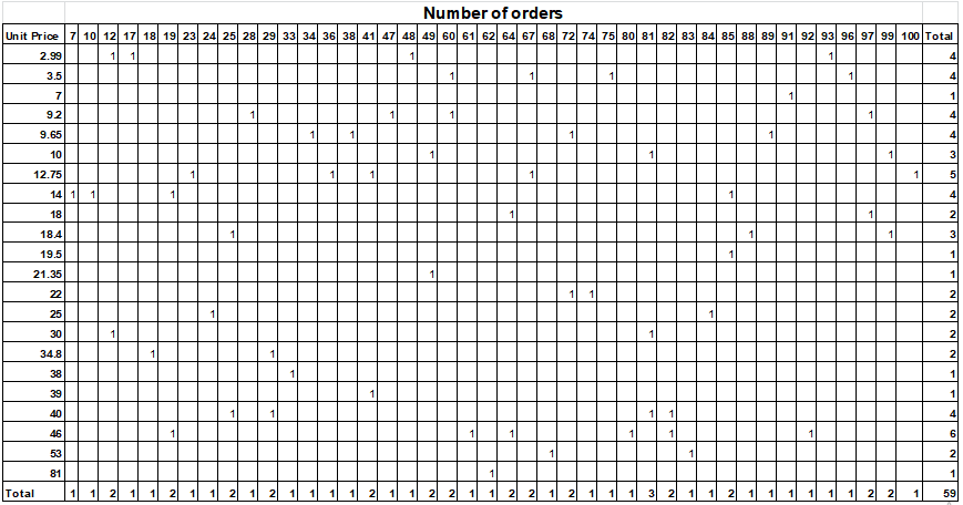
Table 1
Table 1 above shows the distribution of unit price by number of orders. It can be observed that the most frequent unit price was 46 pounds which had a frequency of 6. This was followed by unit price of 12.75 pounds which had a frequency of 5. However, most of the prices had a frequency of 4.
Distribution of revenue by salesperson
| Salesperson | Grand Total |
| Andrea Larsen | £ 14,896.90 |
| Camilla Meerheimb | £ 8,278.07 |
| Caroline Storgaard | £ 17,393.27 |
| Leanne Milner | £ 2,130.25 |
| Roger Bennett | £ 7,572.73 |
| Silvia Gallo | £ 2,612.00 |
| Stella Haydon | £ 15,830.48 |
| Uffe Nielsen | £ 7,951.75 |
Table 2
The table above shows the distribution of revenue by salesperson. It can be observed that Caroline Storgaard had the highest revenue. She had 17,393.27 pounds compared to the rest. She was followed by Stella Haydon who had revenue amounting to 15,830.48 pounds. The third largest revenue was from 14,896.90 pounds. The least revenue was from Leanne Milner who had revenue of 2130.25 pounds.
Distribution by revenue by region
| REGION | REVENUE |
| East | £ 23,174.97 |
| North | £ 23,782.23 |
| South | £ 17,393.27 |
| West | £ 12,314.98 |
| Total | £ 76,665.45 |
Table 3
The table above shows distribution of revenue by region. It can be observed that a bigger percentage of revenue came from East and North region. They had revenue of 23,174.97 pounds and 23,782.23 pounds respectively. The region which contributed the least revenue among the four regions is the west region. The region contributed total revenue of 12,314.98 pounds.
Distribution by revenue by top 5 customers
| Customer Name | Revenue |
| Company D | £ 14,896.90 |
| Company J | £ 9,340.07 |
| Company F | £ 8,049.75 |
| Company A | £ 6,594.03 |
| Company H | £ 6,292.45 |
| Grand Total | £ 45,173.20 |
Table 4
The result of table 4 shows the revenue received by the business from the top five customers. It can be seen that the total revenue of 45,173.20 pounds. The company that contributed the most revenue was Company D. It generated revenue of 14,896.90 pounds. The company that contributed the second most revenue was Company J. It generated revenue of 9,340.07 pounds. The company that contributed the third most revenue was Company F. It generated revenue of 8,049.75 pounds. The company that generated the least revenue for the business was Company H. It generated a total of 6,292.45 pounds.
Distribution by revenue by top 10 categories
| Category | Sum of Revenue |
| Beverages | £ 23,408.30 |
| Dried Fruit & Nuts | £ 12,646.00 |
| Sauces | £ 8,680.00 |
| Jams, Preserves | £ 7,722.00 |
| Canned Meat | £ 3,900.80 |
| Condiments | £ 3,702.00 |
| Candy | £ 3,404.25 |
| Baked Goods & Mixes | £ 3,124.40 |
| Pasta | £ 2,911.50 |
| Soups | £ 2,248.45 |
| Total | £ 71,747.70 |
Table 5
The result of table 5 shows the revenue received by the business from the top ten categories. It can be seen that the total revenue of 71,747.70 pounds. The category that contributed the most revenue was beverage category. It generated revenue of 23,408.30 pounds. The category that contributed the second most revenue was dried fruits and nuts category. It generated revenue of 12,646.00 pounds. The category that contributed the third most revenue was sauces. It generated revenue of 8,680 pounds.
QUESTION TWO
a.
Descriptive statistics for initial purchase amount in pounds
| Initial purchases (in £) | |
| Mean | 1428.111 |
| Standard Error | 67.03144 |
| Median | 1320 |
| Mode | 1490 |
| Standard Deviation | 449.6606 |
| Sample Variance | 202194.6 |
| Kurtosis | 1.465829 |
| Skewness | 0.432633 |
| Range | 2475 |
| Minimum | 175 |
| Maximum | 2650 |
| Sum | 64265 |
| Count | 45 |
| Confidence Level(95.0%) | 135.093 |
| Upper quartile | 1620 |
| Lower quartile | 1200 |
| Interquartile range | 420 |
Table 6
The table above shows the summary statistics for amount of purchases in pounds. The mean purchase amount was 1428.11 pounds with a standard deviation of 449.66 pounds. Most of the purchase amount was 1490 pounds. The least amount of purchase was 175 pounds while the highest amount of purchase made was 2650 pounds. The lower quarter spent 1200 pounds in purchase while the upper quarter of the customers spent 1620 pounds. From the kurtosis value of 1.47, it can be concluded that the purchase amounts were not normally distributed. A normal distribution has a kurtosis value zero or close to zero.
b.
The mean and median are not close to each other so it can be concluded that the data for amount of initial purchase is not normally distributed.
c. 95% confidence interval for the mean
QUESTION THREE
- Scatterplot of advertising amount and revenue
Figure 1
- Correlation coefficient
- Equation of the regression
Regression results
| SUMMARY OUTPUT | ||||||
| Regression Statistics | ||||||
| Multiple R | 0.928343 | |||||
| R Square | 0.86182 | |||||
| Adjusted R Square | 0.844548 | |||||
| Standard Error | 2.95516 | |||||
| Observations | 10 | |||||
| ANOVA | ||||||
| df | SS | MS | F | Significance F | ||
| Regression | 1 | 435.7362 | 435.7362 | 49.89554 | 0.000106 | |
| Residual | 8 | 69.86376 | 8.73297 | |||
| Total | 9 | 505.6 | ||||
| Coefficients | Std error | t Stat | P-value | Lower 95% | Upper 95% | |
| Intercept | 24.99629 | 2.608647 | 9.582089 | 1.17E-05 | 18.98074 | 31.01184 |
| Advertising expenditure (£1,000) | 4.551245 | 0.644317 | 7.063678 | 0.000106 | 3.065448 | 6.037042 |
Table 7
Regression equation
- Regression coefficients
The coefficient of advertising expenditure is 4.55. This means that a unit increase in advertising expenditure causes 4.55 units increase in sales revenue. The p-value for this coefficient is 0.0001. This means that the predictor variable is significant.
- Amount of revenue in sales revenue of £6000?
- Yes I would use the regression model to predict. The value is an independent variable.
| Initial purchases (in £) |
| 1400 |
| 820 |
| 2650 |
| 1680 |
| 900 |
| 1140 |
| 1140 |
| 1720 |
| 1420 |
| 860 |
| 1250 |
| 2350 |
| 2120 |
| 1710 |
| 1490 |
| 1490 |
| 1560 |
| 1180 |
| 1390 |
| 1490 |
| 1320 |
| 1050 |
| 1620 |
| 1260 |
| 1260 |
| 2160 |
| 1270 |
| 1610 |
| 1350 |
| 1720 |
| 2200 |
| 2290 |
| 1290 |
| 1290 |
| 870 |
| 1260 |
| 175 |
| 1270 |
| 1490 |
| 1260 |
| 1210 |
| 1180 |
| 1180 |
| 1720 |
| 1200 |