Introduction

This is an R Markdown Notebook. The dataset in use is Iris dataset. We execute the codes within the notebook and the output is generated beneath the code. The aim of this report is to present an understanding of the relationship between the independent variables. The dependent variable in this problem is Species

Correlation Analysis

In this section, we analyze the correlation between the Species (dependent variable) and other variables.

Screening the variables

iris<-read.csv(“C:\\Users\\310187796\\Desktop\\iris_exams.csv”)
str(iris)

## ‘data.frame’:    300 obs. of  6 variables:
##  $ id          : Factor w/ 300 levels “S001″,”S002”,..: 1 2 3 4 5 6 7 8 9 10 …
##  $ Species     : Factor w/ 3 levels “setosa”,”versicolor”,..: 1 1 1 1 1 1 1 1 1 1 …
##  $ Sepal.Length: num  4.75 5.07 5.24 5.48 4.9 …
##  $ Sepal.Width : num  3.3 3.68 3.44 3.96 2.81 …
##  $ Petal.Length: num  1.44 1.21 1.59 1.53 1.49 …
##  $ Petal.Width : num  0.235 0.111 0.405 0.272 0.345 …

myvars <- c(“Species”, “Sepal.Length”, “Sepal.Width”, “Petal.Length”, “Petal.Width”)
iris <- iris[myvars]
iris$Species<-as.numeric(iris$Species)
attach(iris)
summary(iris)

##     Species   Sepal.Length    Sepal.Width     Petal.Length  
##  Min.   :1   Min.   :4.417   Min.   :1.796   Min.   :1.135  
##  1st Qu.:1   1st Qu.:5.209   1st Qu.:2.720   1st Qu.:1.566  
##  Median :2   Median :5.844   Median :2.992   Median :4.228  
##  Mean   :2   Mean   :5.857   Mean   :3.064   Mean   :3.738  
##  3rd Qu.:3   3rd Qu.:6.448   3rd Qu.:3.375   3rd Qu.:5.205  
##  Max.   :3   Max.   :8.478   Max.   :4.810   Max.   :6.955  
##   Petal.Width      
##  Min.   :-0.03371  
##  1st Qu.: 0.30278  
##  Median : 1.28776  
##  Mean   : 1.19830  
##  3rd Qu.: 1.87452  
##  Max.   : 2.62487

The above output presents the summary data for all the variables in the dataset. From the above findings, it is evident that the average value for the species is 2 with a minimum of 1 and a maximum of 2. There are no missing data points in the dataset neither are there outliers.

Checking for assumptions

In this section we check the assumptions such as linearity, normality and equal variances (homogeneity).

Normality test

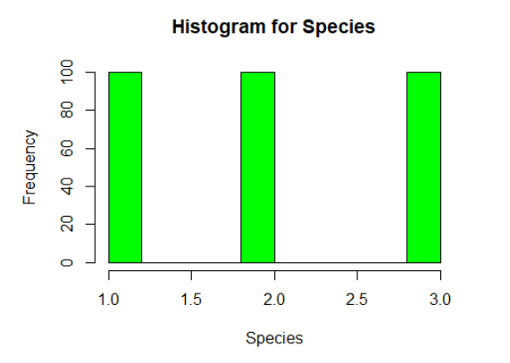
hist(iris$Species, xlab=”Species”, main=”Histogram for Species”, col=”green”)

shapiro.test(iris$Species)

##
##  Shapiro-Wilk normality test
##
## data:  iris$Species
## W = 0.79301, p-value < 2.2e-16

From the output, the p-value < 0.05 implying that the distribution of the data are significantly different from normal distribution. In other words, we can assume the Species are not normally distributed.

Results of the correlation test

The results of the correlation test are presented below.

cor(iris,  method = “pearson”, use = “complete.obs”)

##                 Species Sepal.Length Sepal.Width Petal.Length Petal.Width
## Species       1.0000000    0.7434159  -0.5169396    0.9509344   0.9625907
## Sepal.Length  0.7434159    1.0000000  -0.2002927    0.8534125   0.7893659
## Sepal.Width  -0.5169396   -0.2002927   1.0000000   -0.5302401  -0.4680819
## Petal.Length  0.9509344    0.8534125  -0.5302401    1.0000000   0.9653060
## Petal.Width   0.9625907    0.7893659  -0.4680819    0.9653060   1.0000000

From the above results, it can be seen that strong positive relationship exists between Species and Petal width (r = 0.9626). There was also a strong positive relationship between Species and Petal length (r = 0.9509). A moderately strong positive relationship between Species and sepal length (r = 0.7434). lastly, there was a moderate neagtive relationship between Species and sepal width (r = -0.5169).

Regression analysis

The results of the correlation test are presented below.

mod<-lm(Species~Sepal.Length+Sepal.Width+Petal.Length+Petal.Width, data=iris)
summary(mod)

##
## Call:
## lm(formula = Species ~ Sepal.Length + Sepal.Width + Petal.Length +
##     Petal.Width, data = iris)
##
## Residuals:
##      Min       1Q   Median       3Q      Max
## -0.76982 -0.10135  0.01186  0.11046  0.55591
##
## Coefficients:
##              Estimate Std. Error t value Pr(>|t|)    
## (Intercept)   1.38919    0.13470  10.313  < 2e-16 ***
## Sepal.Length -0.21332    0.03919  -5.444 1.10e-07 ***
## Sepal.Width   0.03303    0.03741   0.883    0.378    
## Petal.Length  0.28771    0.04123   6.978 1.98e-11 ***
## Petal.Width   0.57046    0.06495   8.782  < 2e-16 ***
## —
## Signif. codes:  0 ‘***’ 0.001 ‘**’ 0.01 ‘*’ 0.05 ‘.’ 0.1 ‘ ‘ 1
##
## Residual standard error: 0.1986 on 295 degrees of freedom
## Multiple R-squared:  0.9418, Adjusted R-squared:  0.941
## F-statistic:  1194 on 4 and 295 DF,  p-value: < 2.2e-16

The above results shows that all the predictor variables are significant in the model except sepa width which found to be insignificant in the model (p > 0.05)

Regression analysis with only significant variables

The results of the correlation test are presented below.

mod<-lm(Species~Sepal.Length+Petal.Length+Petal.Width, data=iris)
summary(mod)

##
## Call:
## lm(formula = Species ~ Sepal.Length + Petal.Length + Petal.Width,
##     data = iris)
##
## Residuals:
##      Min       1Q   Median       3Q      Max
## -0.75220 -0.09782  0.00526  0.10802  0.55905
##
## Coefficients:
##              Estimate Std. Error t value Pr(>|t|)    
## (Intercept)   1.41843    0.13052  10.868  < 2e-16 ***
## Sepal.Length -0.19067    0.02962  -6.438 4.87e-10 ***
## Petal.Length  0.26356    0.03085   8.544 6.97e-16 ***
## Petal.Width   0.59515    0.05860  10.156  < 2e-16 ***
## —
## Signif. codes:  0 ‘***’ 0.001 ‘**’ 0.01 ‘*’ 0.05 ‘.’ 0.1 ‘ ‘ 1
##
## Residual standard error: 0.1985 on 296 degrees of freedom
## Multiple R-squared:  0.9417, Adjusted R-squared:  0.9411
## F-statistic:  1593 on 3 and 296 DF,  p-value: < 2.2e-16

From the above output, it is evident that all the three predictor variables are significant in the model (p < 0.05). The overall model is also seen to be significant [F(3, 146) = 648.3, p = 0.000]. The R-squared value is 0.9287; this means that 92.87% of the variation in the dependent variable (Species) is explained by the three predictor variables in the model. The coefficient of sepal length is -0.1907; this implies that a unit increase in the sepal length is expected to result in a decrease in the species by 0.1907. The coefficient of petal length is 0.2636; this implies that incresing the petal length by a unit would result in an increase in the species by 0.2636. Lastly, the coefficient of petal width is 0.5952; this implies that incresing the petal width by a unit would result in an increase in the species by 0.5952.

ANOVA analysis

This section presents ANOVA test with Species as the dependent variable.

anova_one_way <- aov(Species~Sepal.Length, data = iris)
summary(anova_one_way)

##               Df Sum Sq Mean Sq F value Pr(>F)    
## Sepal.Length   1 110.53   110.5   368.2 <2e-16 ***
## Residuals    298  89.47     0.3                   
## —
## Signif. codes:  0 ‘***’ 0.001 ‘**’ 0.01 ‘*’ 0.05 ‘.’ 0.1 ‘ ‘ 1

There was significant effect of Sepal length on Speices at the p<.05 level for the given conditions [F(1, 298) = 368.2, p = 0.000].

T-test analysis

This section presents the t-test with sepal length as the dependent variable. We sought to test the following hypothesis. Null Hypothesis (H0) : Sepal.Length has no effect on Species (Setosa & Versicolor Only). That is to say that the difference between the observed Sepal.Length values for various Species are not statistically different

Alternate Hypothese (HA) : Sepal.Length has some effect on Species (Setosa & Versicolor Only). That is to say that the difference between the observed Sepal.Length values for various Species are in fact different from each other.

iris<-read.csv(“C:\\Users\\310187796\\Desktop\\iris_exams.csv”)
str(iris)

## ‘data.frame’:    300 obs. of  6 variables:
##  $ id          : Factor w/ 300 levels “S001″,”S002”,..: 1 2 3 4 5 6 7 8 9 10 …
##  $ Species     : Factor w/ 3 levels “setosa”,”versicolor”,..: 1 1 1 1 1 1 1 1 1 1 …
##  $ Sepal.Length: num  4.75 5.07 5.24 5.48 4.9 …
##  $ Sepal.Width : num  3.3 3.68 3.44 3.96 2.81 …
##  $ Petal.Length: num  1.44 1.21 1.59 1.53 1.49 …
##  $ Petal.Width : num  0.235 0.111 0.405 0.272 0.345 …

newiris <- subset(iris, Species==“setosa” | Species==“versicolor”)
str(newiris)

## ‘data.frame’:    200 obs. of  6 variables:
##  $ id          : Factor w/ 300 levels “S001″,”S002”,..: 1 2 3 4 5 6 7 8 9 10 …
##  $ Species     : Factor w/ 3 levels “setosa”,”versicolor”,..: 1 1 1 1 1 1 1 1 1 1 …
##  $ Sepal.Length: num  4.75 5.07 5.24 5.48 4.9 …
##  $ Sepal.Width : num  3.3 3.68 3.44 3.96 2.81 …
##  $ Petal.Length: num  1.44 1.21 1.59 1.53 1.49 …
##  $ Petal.Width : num  0.235 0.111 0.405 0.272 0.345 …

t.test(Sepal.Length~Species, data=newiris)

##
##  Welch Two Sample t-test
##
## data:  Sepal.Length by Species
## t = -14.045, df = 157.12, p-value < 2.2e-16
## alternative hypothesis: true difference in means is not equal to 0
## 95 percent confidence interval:
##  -1.0176746 -0.7667257
## sample estimates:
##     mean in group setosa mean in group versicolor
##                 5.093869                 5.986069

From the results presented below, it is evident that there is no significant difference in the sepal length for the Setosa and versicolor species (p > 0.05).