Question 1

Question a

Table 1: Regression result Average monthly temperature and electricity cost

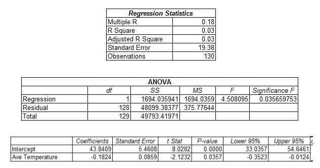
The R square value of the model is 0.03. The value of R square can be interpreted as average temperature accounts only 3 percent variation in cost of electricity. The overall significance of the model can be examined from the significant F value. P value for F statistics is 0.0357 which is less than significance value meaning the model has overall significance. Value of the slope coefficient is -0.1824. This implies cost of electricity decreases by 1.8 percent for every 10-unit increase in average temperature (Gunst 2018). The slope coefficient is statistically significant since the p value of 0.0357 of the coefficient is less than the significance level.

Question b 

Electricity cost with average monthly temperature of 50 F

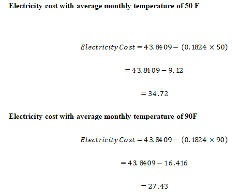
Electricity cost with average monthly temperature of 90F

The predicted electricity cost at a temperature of 90F is lower than that with average monthly temperature of 50F. The lower cost of electricity associated with a relatively high temperature may be due to associated lower cost of appliances used to keep the room warm.

Based on the regression estimate, it is observed that cost of electricity tends to decrease when average temperature goes from very cold to very hot.

Question c 

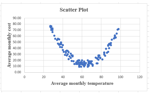
Figure 1: Scatter Plot between average monthly temperature and average monthly cost

The obtained scatter plot suggests a U shaped relation between average monthly temperature and average monthly cost. This explains average monthly cost of electricity first decrease with average monthly temperature, then reaches to the minimum and then starts to increase with increase in monthly temperature.

Question d 

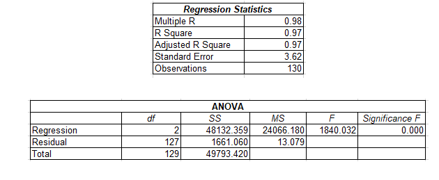
Table 2: Regression result with adding square of average monthly temperature

Question e

The R square value of the new model increases to 0.97. With addition of new variable (average temperature square) the model now accounts 97 percent variation of cost of electricity. Like previous model, the new model has overall significance. The value of the coefficient for average temperature is -6.0944 meaning that cost decreases with increase in average temperature. The coefficient of average temperature square is 0.0481 meaning when average temperature increases at a faster rate electricity cost increases. Both the independent variables are statistically significant.

Question 2 

Question a 

The coefficient of ‘Education’ is 0.0772. The positive regression suggests that with 10-unit increase in education log of wages increases by 0.7 units. In case of age the estimated coefficient is 0.0628. That means with 10 percent increase in age, log of wage increases by 0.6 percent. The regression coefficient of age sqr is -0.00064 (Schroeder, Sjoquist and Stephan 2016). The coefficient suggests that for 10-unit increase in square of age log of wage falls by 0.006 units.

Question b 

Education has a positive effect on wages

Hypothesis

Null hypothesis

Alternative hypothesis

Test statistics

Decision

The critical t value at 5% significance level and 530 degrees of freedom is 1.6477. Computed t value exceeds the critical indicating rejection of null hypothesis. Education therefore has a positive significant impact on wage.

Each year of education adds more than 7% to the yearly wage

Hypothesis

Null hypothesis

Alternative hypothesis

Test statistics

Decision

The critical t value at 5% significance level and 530 degrees of freedom is 1.6477. Computed t value exceeds the critical indicating rejection of null hypothesis (Darlington and Hayes 2016). This supports the claim that education adds more than 7% to the yearly wage.

Question 3 

The possibility that workers with lower ability tend to need more training indicate presence of Multicollinearity problem. Therefore, dropping the variable ‘ability’ is one way to deal with the Multicollinearity problem (Winship and Western 2016). Omitting the variable in turn helps to eliminate Multicollinearity problem giving a more precise and robust estimate for impact of training on productivity.

Question 4

Question a

Table 3: Regression estimate for effect of All Prices on market share of Dubuque company

The coefficient for ‘Price of Dubuque Hot Dogs’ is 0.00076 meaning that market share of Dubuque company decrease by 0.01 percent with 10 percent increase in price of hot dogs. The coefficient for ‘Price of Oscar Mayer’s Hot Dogs’, ‘Price of Ball park regular Hot Dogs’ and ‘Price of Ball park Hot Dogs’ are 0.00026, 0.00035 and 0.00010 respectively indicating that market share of Dubuque company increases with increase in price of hot dogs of its competitors.

Question b 

The sign of coefficient of ‘Price of Dubuque Hot Dogs’ is negative which match the expectation since demand for a product decreases with increase in own price. The coefficient for prices of competitor is positive which explain the impact of price of substitute goods. This is expected as increase in price of competitors’ good increase demand for the concerned good.

Of the four regression coefficients, ‘Price of Dubuque Hot Dogs’ and ‘Price of Oscar Mayer’s Hot Dogs’ are statistically significant (p value is less than 0.05). Rest of the two coefficients are not statistically significant.

Question c 

The problem of multicollinearity exists when the explanatory variables are significantly correlated. In this case Multicollinearity problem may arise of price of Dubuque Hot Dogs is related to any of its competitors’ price or the competitors’ price are interrelated.

Test for suspected collinearity

One popular measure used for detecting severity of Multicollinearity problem is ‘Variance Inflation Factor (VIF)’.  VIF less than 1 meaning low Multicollinearity, VIF between 5 and 10 meaning Multicollinearity is medium and the problem of Multicollinearity is severe is VIF is above 10.

: Coefficient of determination from the regression function.

Table 3: VIF for the explanatory variables

As obtained from the above table VIF for pbreg and pdpbeef are significant high (above 10) meaning that these two variables cause Multicollinearity in the model.

Suggested way to deal with Multicollinearity

• Dropping the correlated variable such as pbreg or pdpbeef
• Taking linear combination of the independent variables (Daoud 2017)
• Partial least square regression analysis or principle component analysis to deal with highly correlated variables

References

Daoud, J.I., 2017, December. Multicollinearity and regression analysis. In Journal of Physics: Conference Series (Vol. 949, No. 1, p. 012009). IOP Publishing.

Darlington, R.B. and Hayes, A.F., 2016. Regression analysis and linear models: Concepts, applications, and implementation. Guilford Publications.

Gunst, R.F., 2018. Regression analysis and its application: a data-oriented approach. Routledge.

Schroeder, L.D., Sjoquist, D.L. and Stephan, P.E., 2016. Understanding regression analysis: An introductory guide (Vol. 57). Sage Publications.

Winship, C. and Western, B., 2016. Multicollinearity and model misspecification. Sociological Science, 3(27), pp.627-649.