Answer to the question 1
Part (a)
Null hypothesis (H0): There is no differences in weight loss between the four groups.
Alternative hypothesis (H1): There is a differences in weight loss between the four groups.
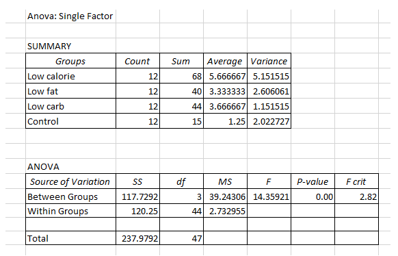
Table 1 ANOVA output
Hence the test statistic (F) = 14.359
It is clear from this test that P-Value < alpha (at 5%). Hence the null hypothesis of this test is rejected. Thus the null hypothesis is significant. At the same time the alternative hypothesis may be accepted. Therefore it may be summarised that there is a differences in the weight loss between the four groups.
Part (b)
Null hypothesis (H0): There is no differences in weight loss between the dieting groups.
Alternative hypothesis (H1): There is a differences in weight loss between the dieting groups.
Table 2 ANOVA output
Hence the test statistic (F) = 6.435
It is clear from this test that P-Value < alpha (at 5%). Hence the null hypothesis of this test is rejected. Thus the null hypothesis is significant. At the same time the alternative hypothesis may be accepted. Therefore it may be summarised that there is a differences in the weight loss between the dieting groups.
Part (c)
From part (a) and (b) it may be concluded that there is a differences in the weight loss between the all the groups. These groups are low calorie, low fat, low carb, and control.
Answer to the question 2
Part (a)
Figure 1 Scatter Plot on Rank versus Mean base Salary
The figure 1 shows the scatter plot on rank versus mean base salary. In this figure in the X-axis represent the rank and in the Y- axis represent the mean base salary. In this scatter plot the rank and the mean base salary shows a linear relationship.
Part (b)
The rank of school is the independent variable and the mean base salary is the dependent variable.
Part (c)
The regression model is homoscedastic.
Part (d)
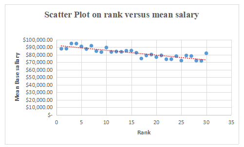
Table 3 Regression output
The coefficient of this model is -644.279.
Part (e)
The regression model is as below
Mean base salary = 92428.73 + (-644.279) * Rank
For school rank = 10
Mean base salary = 92428.73 + (-644.279) * 10
Mean base salary = 92428.73 – 6442.79
= 98871.53
For school rank = 60
Mean base salary = 92428.73 + (-644.279) * 60
Mean base salary = 92428.73 – 38656.8
= 131085.5
Part (f)
Null hypothesis (H0): The estimated coefficient are not significantly different from zero.
i.e. β1 =0
Alternative hypothesis (H0): The estimated coefficient are significantly different from zero.
i.e. β1 0
Test statistic = -8.74
It has been seen that P-value < alpha (at 5% significance level). %). Hence the null hypothesis of this test is rejected. Thus the null hypothesis is significant. At the same time the alternative hypothesis may be accepted. Therefore it may be summarised that the estimated coefficient are significantly different from zero.
Answer to the question 3
Part (a)
In general earning is affected by the education. A person earn much more money when the person is more educated.
Part (b)
Yearly earning = intercept + Education * slope of the education
Part (c)
Figure 1 Scatter Plot on Education versus Earning
The figure 1 shows the scatter plot on education versus earning. In this figure in the X-axis represent the education and the Y-axis represent the earning. The relationship between these two variables is positive but not strong. The sign of the estimated slope is positive, because their relationship is positive.
Part (d)
From this scatter plot on education versus earning it has been seen that most of the assumption on regression has been satisfied. The relation between these two variables are linear. Moreover it is homoscedastic.
Part (e)
Table 4 Regression output
The estimated coefficient of this model = 5728.797
Part (f)
Null hypothesis (H0): The estimated coefficient are not significantly different from zero.
i.e. β1 =0
Alternative hypothesis (H0): The estimated coefficient are significantly different from zero.
i.e. β1 0
Test statistic = 8.0956
It has been seen that P-value < alpha (at 5% significance level). %). Hence the null hypothesis of this test is rejected. Thus the null hypothesis is significant. At the same time the alternative hypothesis may be accepted. Therefore it may be summarised that the estimated coefficient are significantly different from zero.
Answer to the question 4
The scatter plot 1 violate the assumption of linearity. In this scatter plot data points are fallen like U shape in the two dimensional plane. It is nonlinear regression.
The scatter plot 2 violate the assumption of homoscedasticity. The variability of all the data points are not same for all the predicted variable.
The scatter plot 3 violate the assumption of normality. In this scatter plot data points are scattered that is they are no close to the diagonal line.
Answer to the question 5
The regression analysis can be applied to determine the relation between two or more variable. The hypothesis is there is no relation between the variables. Both the primary or secondary data has been applied. The model is as below
Dependent variable = intercept + independent variable or variables* slope of the coefficient or coefficients.
Answer to the question 6
Statement of the problem: To test is there any relationship between the earning and education among 50 sample observations.
Data and source: The data in this study is primary and collected by questionnaire survey method.
Analysis tool and description: The descriptive and inferential statistics has been done in the analysis section. The tool of the analysis is MS-Excel.
Bibliography
Cameron, A.C. and Trivedi, P.K., 2013. Regression analysis of count data (Vol. 53). Cambridge university press.
Cardinal, R.N. and Aitken, M.R., 2013. ANOVA for the behavioral sciences researcher. Psychology Press.
Chatterjee, S. and Hadi, A.S., 2015. Regression analysis by example. John Wiley & Sons.
Gunst, R.F., 2018. Regression analysis and its application: a data-oriented approach. Routledge.
Zhang, J.T. and Liang, X., 2014. One‐way ANOVA for functional data via globalizing the pointwise F‐test. Scandinavian Journal of Statistics, 41(1), pp.51-71.