Introduction
With worsening weather impacting, optimal transportation routes between destinations have never received as much focus as it does today. From the following set of train stations, identify an optimal route from Newcastle to Birmingham. Adverse weather is predicted to move across the country, so calculate alternative routes based on eastern and then western stations being closed. When implemented, we also consider the impact of slower change between trains. What happens to suggested routes when changes take 30 minutes or more?
For a given set of cities like the ones provided in our case, Dijkstra’s Algorithm can be instrumental in trying to establish the shortest distance that connects an initial city to a target city through a number of other cities in between (Javaid, 2013). The algorithm will keep running until it has visited all the reachable cities that have been introduced into the graph. What this means is that after running the algorithm only once, we can locate the shortest path between the cities and save these results for reference in the future. The only time we would have to run their tourism all over again if parameters such as the distance between the cities change (Wang, 2012).
Theory
Dijkstra’s algorithm can be explained as a technique that is used to search and transverse both directed and undirected graphs and determine what path from a starting node to a target node is the most optimal or shortest possible path (Jinhao & Chidong, 2012).
Conditions that have to exist for Dijkstra’s Algorithm to function include;
- All edges must have nonnegative weights
- Dijkstra’s algorithm is appropriate for use with both directed and undirected graphs
- The graph must be connected (Ginting et al., 2019)
Let the node at which we are beginning be known as the starting node. Dijkstra’s algorithm will relegate some starting distance weights and will attempt to make them better bit by bit to establish the most optimal path between the starting city and the ending city (Alam & Faruq, 2019). Set each node a given placeholder and give a value of zero for the starting node and to infinity for every single other node. Check all the unvisited cities or nodes. Set the starting node as the current one and make a lot of the unvisited nodes called the unvisited set comprising of a considerable number of nodes (Mukherjee, 2012). For the present node, consider all its unvisited neighbors and figure their provisional distances. For instance, if the present node is Crewe is set apart with a distance of 30, and the edge interfacing it with a neighbor Birmingham has a distance of 57, at that point, the distance to Birmingham through Crewe is computed by adding 30 to 57.
What makes Dijkstra’s Algorithm special and unique in finding the shortest possible distances between two nodes is because it works for both directed and undirected graphs (Schulz et al., 2011). The algorithm employs the use of a greedy approach wherein every iteration it tries to establish the minimum distance between the connecting cities. On the other hand, one disadvantage of using this algorithm is that it cannot be used with negative weights. In order to improve on this we can use other algorithms such as Bellman-Ford which is much slower but allows us to work with negative weights (Deepa et al., 2018).
Implementation
The algorithm will follow the below steps in searching and traversing the presented graph in order to determine the shortest possible route between Newcastle and Birmingham. Every time that we want to visit the next neighboring city, the algorithm will pick the city that has the shortest known distance and visit it first (Tsai & Chen, 2017).
- When we arrive in the next city that we were set to visit then we will check all its neighboring cities to establish the shortest possible path that connects between our current city and the next city
- For each neighboring city, we will then calculate the distance or in this case the time taken to move from the neighboring cities by adding all the time that we have spent or the weight that is indicated in the edges of these cities and reference it with the starting city – Newcastle (Peyer et al., 2019).
- Finally, if the time taken to move from one city to the next is a known distance like in our case, then we will update the algorithm with the shortest distance that we had on record from the initial starting city.
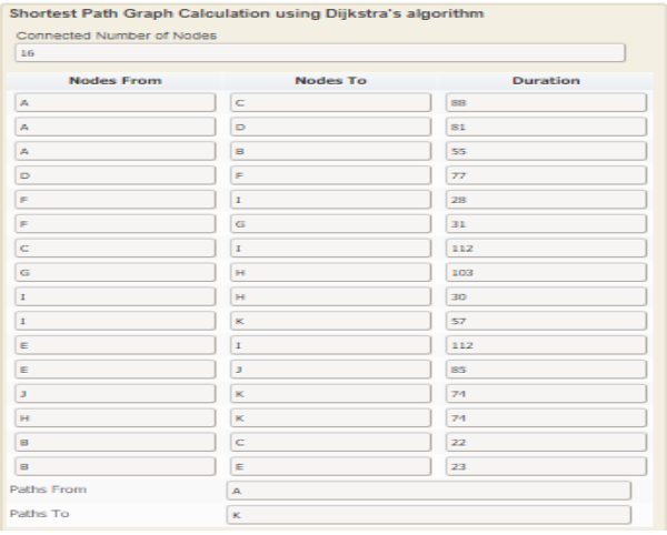
The directed graph

The diagram above shows a weighted graph of cities that are connected. A connection between cities where there is a possible road also includes the weight that is given as the time needed to move from city A to city B. For instance, to move from Newcastle to York, one will take 55 minutes. The directed graph shows all the possible routes that one can use to move from Newcastle to Birmingham with their associated time of moving from one city to the next. According to the graph theory, the weight of a connected graph can be given as the time one will take to move from one city to the other, the capacity of load that can be moved from one city to the other or the distance between the two cities (Schulz et al., 2011).
The optimal path between Newcastle and Birmingham
Represent cities using alphabetical letters
Newcastle – A
York – B
Leeds – C
Carlisle – D
Doncaster – E
Wigan – F
Liverpool – G
Shrewsbury – H
Crewe – I
Nottingham – J
Birmingham -K
The shortest path is calculated as A–>B–>E–>J–>K with a cost of 237 minutes as shown below.

All in all, how could we get that number? It can appear to be befuddling from the start. However, we can separate it into parts. Keep in mind, regardless of which vertex we’re seeing. We generally need to aggregate the shortest known optimal paths from our beginning to our present vertex.
A–>B–>E–>J–>K, which in the case of our cities indicate that we will move from Newcastle -> York -> Doncaster ->Nottingham ->Birmingham. The final weighted cost of the shortest path is calculated by adding the individual weights of paths between the cities, that is,
| From | To | Cost of movement (in minutes) |
| Newcastle | York | 55 |
| York | Doncaster | 23 |
| Doncaster | Nottingham | 85 |
| Nottingham | Birmingham | 74 |
| Total weight | 237 |
Alternative routes
Since we do not know the conditions of the roads, then it is advisable to calculate alternative routes from Newcastle to Birmingham. We also assume that any impassable road is not a road, or a traveler will have prior information about the conditions of the road before deciding on what route to follow.

| Route | Cost |
| Newcastle-> Leeds-> Crewe-> Shrewsbury-> Birmingham | 88 + 112 + 30 + 74 = 304 |
| Newcastle-> Leeds-> Crewe -> Birmingham | 88 + 112 + 57 = 257 |
| Newcastle-> Caelisle-> Wigan-> Liverpool-> Shrewsbury-> Birmingham | 81 + 77 + 31 + 103 + 74 = 366 |
| Newcastle-> Caelisle-> Wigan ->Crewe-> Shrewsbury-> Birmingham | 81 + 77 + 28 + 30 + 74 = 290 |
| Newcastle-> Caelisle-> Wigan ->Crewe -> Birmingham | 81 + 77 + 28 + 57 = 243 |
| Newcastle-> York-> Leeds-> Crewe-> Shrewsbury-> Birmingham | 55 + 22 + 112 + 30 + 74 = 293 |
| Newcastle-> York -> Leeds-> Crewe -> Birmingham | 55 + 22 + 112 + 57 = 246 |
| Newcastle-> York -> Doncaster-> Crewe-> Shrewsbury-> Birmingham | 55 + 23 + 112 + 30 + 74 = 294 |
| Newcastle-> York -> Doncaster ->Crewe -> Birmingham | 55 + 23 + 112 + 57 = 247 |
Slower changing times
For any other conditions apart from the time taken to move from one city to the next, Dijkstra’s Algorithm may prove difficult or unfeasible to use. Here, we would want an intelligent algorithm that can combine some factors such as slow-changing time between trains, traffic jams, or an instance where the traveler decides to buy something or stop at some point in their journey. For instance, GoogleMaps systems combine real-time data and can see traffic, know the road condition (like a hill). Using all these conditions and intelligent systems, it can give you the shortest route and other alternative routes (Deepa et al., 2018). In simpler terms, the changing time, for instance, 30 minutes, if constant for every time one is changing a train, then it should be added to the total time of the journey. This will not affect which route is optimal.
Conclusion
In conclusion, the report has implemented Dijkstra’s Algorithm to find the optimal route between Newcastle and Birmingham. From all the above-calculated weights of alternative routes have higher values than the one for the optimal path. This is a verification that our optimal path is the shortest path between Newcastle and Birmingham.
References
Alam, M. A., & Faruq, M. O. (2019). Finding Shortest Path for Road Network Using Dijkstra’s Algorithm. Bangladesh Journal of Multidisciplinary Scientific Research, 1(2), 41–45. https://doi.org/10.46281/bjmsr.v1i2.366
Deepa, G., Kumar, P., & Manimaran, A. (2018). Dijkstra Algorithm Application: Shortest Distance between Buildings. International Journal of Engineering & Technology, 7(4.10), 974–976. https://doi.org/10.14419/ijet.v7i4.10.26638
Ginting, H. N., Osmond, A. B., & Aditsania, A. (2019). Item Delivery Simulation Using Dijkstra Algorithm for Solving Traveling Salesman Problem. Journal of Physics: Conference Series, 1201, 012068. https://doi.org/10.1088/1742-6596/1201/1/012068
Javaid, M. A. (2013). Understanding Dijkstra Algorithm. SSRN Electronic Journal. https://doi.org/10.2139/ssrn.2340905
Jinhao, & Chidong. (2012). Research of shortest path algorithm based on the data structure. 2012 IEEE International Conference on Computer Science and Automation Engineering, 108–110. https://doi.org/10.1109/ICSESS.2012.6269416
Mukherjee, S. (2012). Dijkstra’s Algorithm for Solving the Shortest Path Problem on Networks Under Intuitionistic Fuzzy Environment. Journal of Mathematical Modelling and Algorithms, 11(4), 345–359. https://doi.org/10.1007/s10852-012-9191-7
Peyer, S., Rautenbach, D., & Vygen, J. (2019). A generalization of Dijkstra’s shortest path algorithm with applications to VLSI routing. Journal of Discrete Algorithms, 7(4), 377–390. https://doi.org/10.1016/j.jda.2007.08.003
Schulz, F., Wagner, D., & Weihe, K. (2011). Dijkstra’s algorithm on-line: An empirical case study from public railroad transport. Journal of Experimental Algorithmics, 5, 12–es. https://doi.org/10.1145/351827.384254
Tsai, P.-S., & Chen, J.-Y. (2017). Combining turning point detection and Dijkstra’s algorithm to search the shortest path. Advances in Mechanical Engineering, 9(2), 1687814016683353. https://doi.org/10.1177/1687814016683353
Wang, S.-X. (2012). The Improved Dijkstra’s Shortest Path Algorithm and Its Application. Procedia Engineering, 29, 1186–1190. https://doi.org/10.1016/j.proeng.2012.01.110