Abstract
This paper aims at determining the factors that predict the price of the house. This is crucial information that is relevant to the real estate industry. The data concerning the real estate price prediction was obtained from the Kaggle website. The data contained seven variables and 415 observations. The model created showed that age, location, and size of the house affect the price of the homes. The model also showed that older houses tend to be cheaper. Also, the houses that had a higher number of stores were much expensive, and lastly, the houses which are near stations were expensive.
2.0 Introduction
A lot of people tend to engage them in real estate business because they believe that business is a big deal. It one of the businesses that people perceive as a safe investment. However, the business has been affected by several influences such as diseases, etc. Take, for instance, the COVID-19 pandemic has made the individual who has engaged in the real estate business to make a lot of loss. This is because the investors who own business buildings are at a higher risk of getting losses since enterprises have closed down. This is one of the unfortunate situations that have occurred. However, they are a lot of benefits it can get if everything is stable. Real estate business people enjoyed a vast wealth from the properties they have invested in. It is one of the businesses that can make a person earn all his lifetime. The price of the houses tends to rise over time. Only in a rare situation do we find that the value of homes has depreciated, e.g., during disasters. When the demand for home increases, then the costs of homes increased. Homes located in emerging towns tend to be much expensive compared to the other regions which are not well developed. The demand for houses is high in such areas. This is one of the factors that lead to an increase in the price in such regions. This means that the prices of homes vary from region to parts. This paper is crucial to those investors and people who want to learn how the prices of the homes fluctuate the reason why they fluctuate. This will increase their knowledge in the field of real estate. The rate of the mortgage is one of the factors that can determine the selling price of the house from the seller. When the mortgage rate is low, the price of the homes will tend to be lower.
3.0 Background
3.1: Previous models
There are several factors that can predict the price of the houses; different scholars have developed machine learning techniques that can accurately predict the price of the house. Some scholars have used the housing price index with the price of the house to create a model that is able to predict the price of the house. The model aimed at helping the real estate agents to make better decisions when deciding on the price of the house (Park & Bae, 2015; Sarip, Hafez & Daud, 2016; Wang et al. 2014).
3.2: Factors affecting the price of the houses
A large house tends to be more expensive. The size of the house is categorized with features such as the number of bedrooms, bathrooms, etc. Also, houses age is crucial in determining the price of the house. The quality of constructions and the level of renovation are associated with the age of the houses. Houses have quality constructions and highly renovated are much expensive compared to ordinary houses. The location of the houses plays a major role in determining the price houses, houses which are located near towns, or transportation stations are much expensive. The depreciation of houses varies according to the region of the house, the market trends, and the age distribution of the houses. There are some temporal factors that affect the price of the house, and these factors include market trends. The inflation might affect the price of the houses making the prices go up and vice versa (Huang, Wu & Barry, 2010; Mian, & Sufi, 2011; Basten & Koch, 2015).
4.0 Methodology
4.1 Data
The data that was used for the research contained information about the real estate. The data was obtained from the Kaggle website (https://www.kaggle.com/quantbruce/real-estate-price-prediction). The data contained seven variables and 414 observations. The variables of the real estate data were;
- X1 – The date at which the property was sold
- X2 – The age of the house
- X3 – the distance of the house to the nearest MRT station
- X4 – number of convenience stores
- X5 – latitude
- X6 – longitude
- Y – house price per unit area
Dependent variable = y
Independent variable = X2, X3, X4,
4.2 Methodology
The data will be analyzed in Excel statistical tool. The descriptive statistics of the age of the house, the distance of the house to the nearest MRT station, the number of convenience stores, and the price of the house per unit area will be determined. The price of the house per unit area will be the dependent variable, while the remaining variables will be the independent variables. The correlation analysis of the variables will be determined to check the relationship between the variables. Regression analysis will be conducted to determine whether the age of the house, distance to the nearest MRT station, number of convenience stores (independent variables) have a significant effect on the price of the house per unit area.
The hypothesis that will be tested using excel is
H 0 – There is no significant relationship between the dependent and independent variable
H 1 – There is a significant relationship between the dependent and independent variable
5.0 Results
5.1 Descriptive Statistics
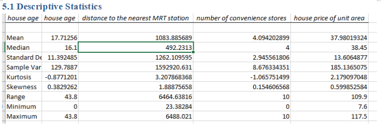
The table shows that the average house age of the data was 16.1 (SD = 11.39). The average distance to the nearest MRT station was 1083 m (SD = 1262.11). The average number of conveniences stores was 4 (SD= 2.9), and finally, the average house price per unit area was $37.98 (SD= $ 13.6).
5.2: Correlation Analysis
Table 2.1: Correlation Analysis
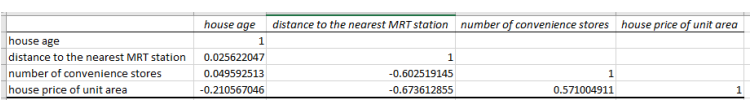
The relationship between the age of the house and the price of the house per unit area was obtained to be negative and low (21.05 %). This means that the older the house, the less the price of the house. The relationship between the house price of per unit area and the distance of the house to the nearest MRT station was negative and strong (67.36 %). This means when the houses near MRT station are more expensive than those which are farther from the MRT station. The relationship between the price of the house and the number of conveniences was positive but very low (4.9%). Meaning the higher the number of conveniences stores the higher price of the house.
Fig 1.2: Scatter plot of the house price against the age of the house
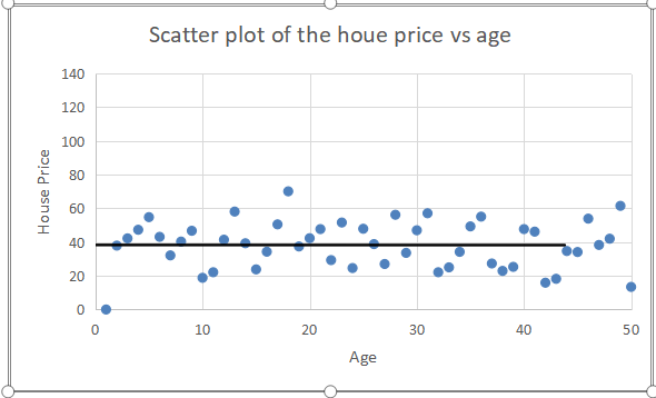
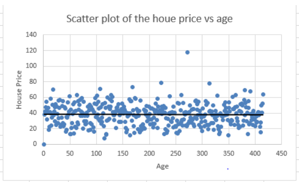
Fig 1.2: Scatter plot of the house price against the distance from the MRT station
5.3: Regression analysis
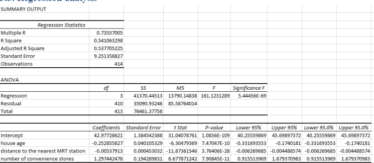
The regression equation can be summarized as
House price = 42.98 – 0.25 (age) – 0.0054 (distance from MRT station) + 1.297 (number of conveniences stores)
The model suggests that a unit increase in the age of the house reduces the price of the houses by 0.25. A unit increase in the distance from MRT station reduces the house price by 0.0054. A unit increase in the number of conveniences stores increases the price of the house by 1.297. The model explained 54.11 % explained the variation of the house price. The model showed a significant effect on the price of the house, i.e., p (5.44e-69 <0.05), meaning that the independent variables had a significant effect on the price of the house.
6.0 Discussion
The obtained model showed that the age of the house had a significant influence on the price of the house. Also, an increase in the age of the house reduces the price of the house. According to Hiller & Lerbs (2016), the houses obtained in the aging urban centers were depreciating in the price due to the depreciation in the quality of the houses. Also, the model showed that the size of the house has a significant effect on the price of the house. Most of the clients prefer houses that have a good size, which is quite expensive compared to the other houses (Ludwig et al. 2019; Kaplan, Mitman & Violante, 2017). Houses which are close to the cities or stations tend to be more expensive. The same concepts have been obtained from the model. Thus the location of the house is so crucial in determining the price of the house (Stroebel & Vavra, 2019; Heyman & Sommervoll, 2019; Theisen & Emblem, 2018).
7.0 Conclusion
The research has successfully explained the factors that predict the price of the house. These have been obtained from both the literature review and analysis. The above information is crucial in determining and predicting the price of the houses. However, future research should be conducted to determine other factors that significantly influence the price of the house. The model created was only able to predict a 54 % variation of the price of the house.
8.0 References
Basten, C., & Koch, C. (2015). The causal effect of house prices on mortgage demand and mortgage supply: Evidence from Switzerland. Journal of Housing Economics, 30, 1-22.
Heyman, A. V., & Sommervoll, D. E. (2019). House prices and relative location. Cities, 95, 102373.
Hiller, N., & Lerbs, O. W. (2016). Aging and urban house prices. Regional Science and Urban Economics, 60, 276-291.
Huang, B., Wu, B., & Barry, M. (2010). Geographically and temporally weighted regression for modeling spatio-temporal variation in house prices. International Journal of Geographical Information Science, 24(3), 383-401.
Kaplan, G., Mitman, K., & Violante, G. L. (2017). The housing boom and bust: Model meets evidence (No. w23694). National Bureau of Economic Research.
Ludwig, A., Mankart, J., Quintana, J., Wiederholt, M., & Vellekoop, N. (2019, February). House Price Expectations and Housing Choice. In 2019 Meeting Papers (No. 848). Society for Economic Dynamics.
Mian, A., & Sufi, A. (2011). House prices, home equity-based borrowing, and the US household leverage crisis. American Economic Review, 101(5), 2132-56.
Park, B., & Bae, J. K. (2015). Using machine learning algorithms for housing price prediction: The case of Fairfax County, Virginia housing data. Expert Systems with Applications, 42(6), 2928-2934.
Sarip, A. G., Hafez, M. B., & Daud, M. N. (2016). Application of fuzzy regression model for real estate price prediction. Malaysian Journal of Computer Science, 29(1), 15-27.
Stroebel, J., & Vavra, J. (2019). House prices, local demand, and retail prices. Journal of Political Economy, 127(3), 1391-1436.
Theisen, T., & Emblem, A. W. (2018). House prices and proximity to kindergarten–costs of distance and external effects?. Journal of Property Research, 35(4), 321-343.
Wang, X., Wen, J., Zhang, Y., & Wang, Y. (2014). Real estate price forecasting based on SVM optimized by PSO. Optik, 125(3), 1439-1443.
Project Description
A report is represented which revolves around the prediction of specific crime categories. The provided data is Chicago crime data, which will be predicted and analyzed with the help of STATISTICA Text miner. This miner is STATISTICA Data Miner’s optional extension, which is perfect to translate the unstructured text data into valuable and meaningful, clusters of decision-making.
Therefore, the real-world data comprises of various forms, and there is guarantee to have an organized or easy to analyze data. Additionally, the data sources could be large. This is where the STATISTICA text miner helps to present the underlying information. It ensures optimization and data enhancing for such data.
STATISTICA Text Miner
STATISTICA Text Miner is mainly developed as a basic and open-architecture tool to ensure text mining the unstructured information. The text miner software is completely integrated into STATISTICA (“STATISTICA Text Miner”, 2020). It isn’t any stand-alone product that is developed by the vendor and linked with STATISTICA. The functionality of text mining is integrated in the workspace environment of STATISTICA Data Miner, STATISTICA Enterprise, or the application of custom STATISTICA.
As large portion of data in the data set is unstructured, the reliable help is provided by text mining to analyze the data patterns, which were missing earlier, for instance, when the feature analysis outlines crimes’ top predictor variables, it can even be beneficial for understanding the particular type of crimes. Therefore, instead of seeing crime as a large category, it is essential to view the particular crime types like theft, assault, and kidnapping. Hence, text mining permits the users to analyze unstructured data, then to produce the lift charts for every single crime types to have deeper understanding.
To perform STATISTICA text mining ensure that the following instructions are followed:
Initially begin with openning the Crime Map data and visit “Text Mining” from the “Data mining” as demonstrated below (Marques De Sa, 2014).
Afterwards, select the variables for Text minig which contains the text by clicking on the Text variable as presented below.
In the text variable selection wizard, select the options “Primary Description”, “Secondary Description”, including the “Location Description” and press on Ok as demonstrated below.
Then, press the OK button, and then select Index. Afterwards, the next screen that displays is the key keywords, followed by the total times they are visible in the dataset as demonstrated below.
Further, in the Result wizard, select Inverse Document Frequency option, next opt “Concept Extraction” tab as presented below.
For Concept Extraction, it is required to perform singular value decomposition by clicking “Perform Singular Value Decomposition.”
Press Screen Plot option which provides the below graph.
These 4 concepts explains thirty percent of the cases, where the number decreases as there is increase in concepts. Thus, the first four concepts are selected for this analysis. Visit “Text Mining” results screen and press “Save Results” tab. Here, variable amount must be changed as 4. Then, press “Append Empty Variables”, as demonstrated below.
Click on Write back current results, which is used to include the new four variables to the variables list for this analysis by selecting Concepts 1, concepts 2, concept 3 and concepts 4. Further, select NewVar1, NewVar2, NewVar3 and NewVar4. Then, click on “Assign” and OK as presented below.
Boosted Trees
The Boosted trees will be created by clicking on Data Mining à select Boosted Trees as demonstrated below.
On Boosted trees, select Classification Analysis and then click on OK as presented below.
Select the variables for the boosted trees by clicking on test variables as presented below.
Then, click on Primary Description variables to be the dependent variable. In continuous variables column, include new variables that are retrieved from text mining. They include – “Concept 1, 2, 3, and 4 as shown below.
Enter the Ok option and it starts STATISTICA for figuring the boost trees as displayed below.
When STATISTICA computation is finished, it gives Boosted Tree Result screen and then visit the Classification tab.
In classification tab, select Lift Chart to provide the results for lift which occurs when text mining is applied to this model as demonstrated below.
The lift chart results are presented below.
The results page show that with text mine option, the unstructured data is enhanced for predicting particular types of crime, for instance, for “Assault,” the prediction ability has been improved with 10 factor, in contrast to the baseline model.
To ensure effective visualization of data i.e., lift charts, it is allowed to merge the graphs. The user can either merge all the graphs to check the specific crime is the highest lift, or could compare more than two graphs simultaneously based on the project’s requirement. Use the right click option for merging the graph, where an option called “merge graph” appear.
Press ok option. Next, once the selection is completed right lift chart. The below graph shows the result.
The user have an option of editing the key by using the right-click option and choosing the Title Properties.
It is possible that a key is re-label by discarding one baseline, including model renaming as “Assault 1.”
It is also possible to modify the line’s colour by choosing each line and right clicking on each, this will ensure that a small window to pop up. Further, proceed by selecting “properties,” and click on “line,” and choose the required colour.
This allows the users to view the positive impact of text mining on the predictive ability for some specific type of crimes. The feature selection finds out the top 3 variables for crime. It is a beneficial analysis for the Chicago Police Department to form the necessary strategies to target their efforts of law enforcement.
Conclusion
It is concluded that the crime data is analyzed effectively with the help of STATISTICA Data Miner and STATISTICA Text Miner. The related instructions and screenshots are included in the report.
References
Marques De Sa, J. (2014). Applied statistics using spss, statistica, matlab and r. New York: Springer.
STATISTICA Text Miner. (2020). Retrieved 23 April 2020, from https://statisticasoftware.wordpress.com/2013/09/18/statistica-text-miner/