Problem 1
| Temperature | Frequency | Cumulative % |
| 62 | 0 | 0.00% |
| 64 | 0 | 0.00% |
| 66 | 2 | 10.53% |
| 68 | 2 | 21.05% |
| 70 | 2 | 31.58% |
| 72 | 3 | 47.37% |
| 74 | 3 | 63.16% |
| 76 | 1 | 68.42% |
| 78 | 5 | 94.74% |
| 80 | 1 | 100.00% |
| 82 | 0 | 100.00% |
| More | 0 | 100.00% |

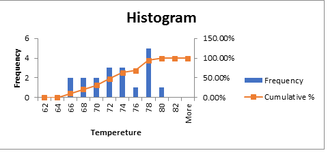
Figure 1: A frequency distribution table for mean temperature in Boston
The distribution has a long tail to the left, hence it is skewed to the left.
| Year(n) | Mean (x) | x^2 | p(x) | x.p(x) | x^2.P(x) |
| 1998 | 72 | 5184 | 0.04955 | 3.56779 | 256.881 |
| 1999 | 69 | 4761 | 0.04749 | 3.27667 | 226.090 |
| 2000 | 78 | 6084 | 0.05368 | 4.18720 | 326.602 |
| 2001 | 70 | 4900 | 0.04818 | 3.37233 | 236.063 |
| 2002 | 67 | 4489 | 0.04611 | 3.08947 | 206.994 |
| 2003 | 74 | 5476 | 0.05093 | 3.76875 | 278.888 |
| 2004 | 73 | 5329 | 0.05024 | 3.66758 | 267.734 |
| 2005 | 65 | 4225 | 0.04474 | 2.90778 | 189.006 |
| 2006 | 77 | 5929 | 0.05299 | 4.08052 | 314.200 |
| 2007 | 71 | 5041 | 0.04886 | 3.46937 | 246.326 |
| 2008 | 75 | 5625 | 0.05162 | 3.87130 | 290.348 |
| 2009 | 68 | 4624 | 0.04680 | 3.18238 | 216.402 |
| 2010 | 72 | 5184 | 0.04955 | 3.56779 | 256.881 |
| 2011 | 77 | 5929 | 0.05299 | 4.08052 | 314.200 |
| 2012 | 65 | 4225 | 0.04474 | 2.90778 | 189.006 |
| 2013 | 79 | 6241 | 0.05437 | 4.29525 | 339.325 |
| 2014 | 77 | 5929 | 0.05299 | 4.08052 | 314.200 |
| 2015 | 78 | 6084 | 0.05368 | 4.18720 | 326.602 |
| 2016 | 72 | 5184 | 0.04955 | 3.56779 | 256.881 |
| 2017 | 74 | 5476 | 0.05093 | 3.76875 | 278.888 |
| Sum of Temp | 1453 | ||||
| µ | 72.8968 | ||||
| Std | 4.2341 | ||||
| Max | 79 | ||||
| Min | 65 | ||||
| Range | 14 | ||||
| ∑p(x) | 1 | ||||
| ∑X^2.P(x) | 5331.5148 |
The data above is normally distributed because the sum of individual probabilities is 1.
b) An outlier can be defined as an observation point which is distant from the rest of the observations.
c)
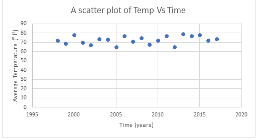
To identify outliers, we would plot a scatter plot of average temperature against time(years).

Figure 2: A scatter plot for mean temperature data in Boston.
From the above figure, it is evident that there are no outliers’ data.
d)

Given, µ=73.0 ,
Now computing the test statistics using the formula
Now P(Z<
Then, P(Z>
Therefore, the what is the probability that the mean will be over 76 in any given
July is .
e)
Given the following values.
µ=73.0 ,
Using the formula to compute test statistics
Now we can compute P(Z<
Computing P(Z>
Therefore, the probability that the mean will be over 80 in any given July is
Problem 2
| Temp Range | Frequency | Cumulative % |
| 82 | 0 | 0.00% |
| 84 | 1 | 5.26% |
| 86 | 4 | 26.32% |
| 88 | 4 | 47.37% |
| 90 | 5 | 73.68% |
| 92 | 5 | 100.00% |
| 94 | 0 | 100.00% |
| 96 | 0 | 100.00% |
| More | 0 | 100.00% |
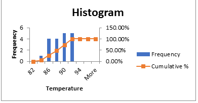
Figure 3: A frequency graph for heatwave temperature.
From the given heat wave data, the following calculations are obtained.
| Days(n) | Temp (x) | p(x) | x.p(x) |
| 1 | 93 | 0.05234 | 4.867192 |
| 2 | 88 | 0.04952 | 4.357907 |
| 3 | 91 | 0.05121 | 4.660101 |
| 4 | 86 | 0.04840 | 4.162071 |
| 5 | 92 | 0.05177 | 4.763084 |
| 6 | 91 | 0.05121 | 4.660101 |
| 7 | 90 | 0.05065 | 4.558244 |
| 8 | 88 | 0.04952 | 4.357907 |
| 9 | 85 | 0.04783 | 4.065841 |
| 10 | 91 | 0.05121 | 4.660101 |
| 11 | 84 | 0.04727 | 3.970737 |
| 12 | 86 | 0.04840 | 4.162071 |
| 13 | 85 | 0.04783 | 4.065841 |
| 14 | 90 | 0.05065 | 4.558244 |
| 15 | 92 | 0.05177 | 4.763084 |
| 16 | 89 | 0.05008 | 4.457513 |
| 17 | 88 | 0.04952 | 4.357907 |
| 18 | 90 | 0.05065 | 4.558244 |
| 19 | 88 | 0.04952 | 4.357907 |
| 20 | 90 | 0.05065 | 4.558244 |
| n=20 | Sum 1777 | 1 | 88.922341 |
| Mean | 88.85 |
| Median | 89.5 |
| Mode | 88 |
| n | 20 |
| Max | 93 |
| Min | 84 |
| Range | 9 |
The data has a normal distribution because mean, median and mode are fairly the same.
Heat wave ~three or more days with a high temperature over 90 degrees Fare height.
P(n≥10)=P(n=12)*p(n=15)*p(n=18)
P(n≥10)= 0.04840 *0.05177 *0.05065=0.0001269
The probability that the heat wave will have a temperature more than 90 in three interval days is 0.0001269
Problem 3
a) The situation of the customers’ behavior exactly fits the parameters for a binomial distribution. This is because of exactly 2 possible outcomes of occurrences from the customers’ behavior to either buy online or from the physical store. There is no any other possible alternative among customers in the market, despite when the occurrence is repeated on multiple times.
b) P (customers purchase online) =40%
=40/100
=0.4
P (Customers purchase from the physical store )=60%
=60/100
=0.6
c) P (Exactly four sales bought online each day =4/12
=1/3
0.3333.
d) P (From 12 sales made each day, fewer than 6 are made online=1-P(6 sales are made online)
=1-6/12
=1-0.5
=0.5
e) From the 12 sales made each day more than 8 are made online =1-P(8sales are made online)
=1-8/12
=1-2/3
=1/3
=0.3333.
Problem 4
a)
My company of choice is Apple Company. According to an article written by Adrian Kinsley on December 29 2018, Apple company made it clear that it would no longer report on iPhone, iPad and mac books unit sales as their objective is to make great products for customer satisfaction. However, this had sparked fears among Apple investors who are now believing that things are not going well for the company. This is because both the iPhone and smartphone sales have been weakening as people no longer buy the iPhone their new features but rather than but rather to change the older used phones. Smartphones have also become dull and Apple is keen on coming up with more exciting features. Together with trump tariff of 10%, tariff increment on Chinese made phones and mac books. Considering the above problems facing the company, Apple has a lot to do in convincing the customer to buy their expensive iPhones so as to maintain a constant revenue (Kinsley, 2018).
b)
I would carry out market analysis research.
The data to be collected Customer’s age, Customer’s Income, region etc.
c)
The data would be a poison’s distribution.
This is because the collected data are both discrete and continuous.
d)
Customers’ buying trends and customer’s average age that use iPhone.
e)
The aim of every business is to make
profits while providing quality products to their esteem customers. Once, the
customer is satisfied with the product, their willingness to pay even for
higher costing products increases. The company, therefore, needs to provide
funds for data collection and analysis failure to which the company will incur
losses.
Refence
Livak, K. J., & Schmittgen, T. D. (2001). Analysis of relative gene expression data using real-time quantitative PCR and the 2− ΔΔCT method. methods, 25(4), 402-408.
Ramakers, C., Ruijter, J. M., Deprez, R. H. L., & Moorman, A. F. (2003). Assumption-free analysis of quantitative real-time polymerase chain reaction (PCR) data. Neuroscience letters, 339(1), 62-66.
A. K. (2018, December 29). Challenges fcing Apple in 2019. Hughes for Hardware 2.0.