Report on Quantitative Methods
Quantitative methods in statistics involve the use of numerical values and is acquired via counting or measuring. To solve quantitative methods, several statistical techniques can be used, in this case, histograms, regression tests, descriptive statistics tests as well as time series analysis are applied. The whole work was done via Microsoft Office Excel 2013.
Question One
In order to find the frequency and display the results for the values of the utility charge, a histogram is applied.
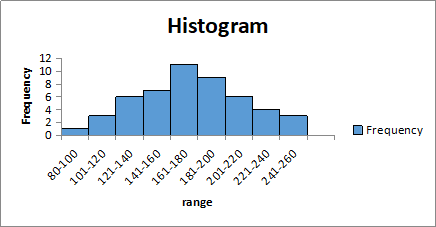
Fig 1. Histogram for utility.
From the histogram, the group with the highest utility numbers is that of 161-180, 11, while the group with the lowest utility is that for 80-100, 1.
Question two
From a survey of 50 undergraduate students descriptive statistics test was done for salary, text books, club affiliation, GPA and student ages to enable answer the following questions,
- The average expected value of salary is 56.76
- Median amount spent on text books is 540.00
- Mode with respect to club affiliation is 0
- Standard deviation for GPA is 0.3996
- Based on variance and standard deviation of the two, spending on textbooks with mean of 564.84, (SE=163.1772) has got high variation compared to the student ages with mean of 20.92 (SE=3.932).
Question three
For the question about rent and the square feet, a scatter plot and regression analysis were conducted to help answer the questions below,
- The scatter plot for rent vs size is shown below.
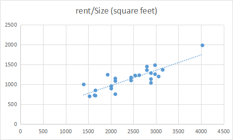
Fig 2. Scatter for Rent vs Square
The plot shows that rent is positively correlated to the house size. The scatter dots are close to the trending line indicating that the two variables are highly related.
- The Equation for the least square regression line is,
- The 90% confidence intervals for both rent and square size are,
| mean | 2427.2 | 1135.32 |
| Confidence level (90%) | 216.9956106 | 98.77158591 |
| lower | 2210.204389 | 1036.548414 |
| upper | 2644.195611 | 1234.091586 |
In other words,
This implies that the values of rent lies between €2210.20 and €2644.20 while square feet values lie between 1036.55 and 1234.09.
- In a case of 1000sqr feet, the rent is,
- Models require varying values for prediction. However, this is not the case here as there is a constant 500ft value indicating that the answers will be the same.
- For the two apartments, I will opt for the 1000ft at €2150 over 1200ft for €2600. This is because the figure 2150euros is less than the per feet figure that is 2173.182 for 1000ft whereas 2600euros is greater than the 2548.076 for 1200ft.
Question Four
This question involved suing dummies to calculate the regression for the Lumber land Ltd softwood demand in the USA. A further time series graph as well as future prediction are done.
- Linear regression with dummies is partly shown in the table below.
| Coefficients | Standard Error | t Stat | P-value | |
| Intercept | 62688 | 4859.066 | 12.90125 | 7.16E-10 |
| 1st Qtr | -106 | 6871.757 | -0.01543 | 0.987883 |
| 2nd Qtr | 2612 | 6871.757 | 0.380107 | 0.708865 |
| 3rd Qtr | 10276 | 6871.757 | 1.495396 | 0.154273 |
=
From the analysis, there is no significant association,, between the demand of Lumber Land Ltd softwood in the USA and the different seasons as the quarterly p-values are greater than 0.05. This is also proven by the small value of the r squared which is 0.159 indicating the small correlation between seasons and demand.
- A Plot of the observed values as well as the expected values is shown below.
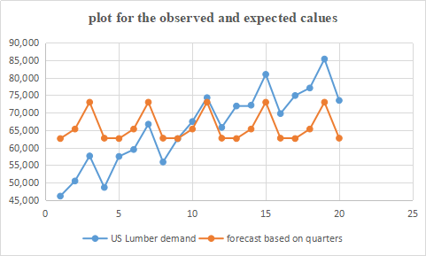
Fig 3. Graph for observed and expected values
From the graph, there is a zigzag (up and down) movements for both the demand and forecast values. The demand line, however, appears to be moving upwards while the forecast line maintains a line.
- To predict for the next four quarters, that’s 2020, dummy variables are created as shown in the table below.
| Qtr 1 | Qtr 2 | Qtr 3 | Quarterly values | |||
| 2020 | Quarter | 1 | 1 | 0 | 0 | 62582 |
| 2 | 0 | 1 | 0 | 65300 | ||
| 3 | 0 | 0 | 1 | 72964 | ||
| 4 | 0 | 0 | 0 | 62688 |
In other words, the quarterly prediction calculation is shown below,
Question Five
This is a maximization problem where the management of a handbag production company is considering using an under-utilised machine to produce a type of cloth handbag and a type of leather handbag. The available time is estimated to be 120 and 50 machine hours per week for machines A and B respectively. The firm needs 4 hours of machine A and 3 hours of machine B to produce 1 cloth handbag and 3 hours of machine A and 1 hour of machine B to produce a single leather handbag.
The sales department predicts an estimated net profit of $30 from the cloth handbag and $50 from the leather handbag.
- Formulating the linear programming problem
The linear programming is formulated as follows;
Let x be the number of units of cloth handbags produced
Let y be the number of units of leather handbags produced
Objective function of the firm is given as follows;
Max: 30x+50y
Constraints on the firm are as follows;
s.t:
4x+3y<=120
3x+y<=50
Non-negativity constraints are as follows ;
x>=0, y>=0
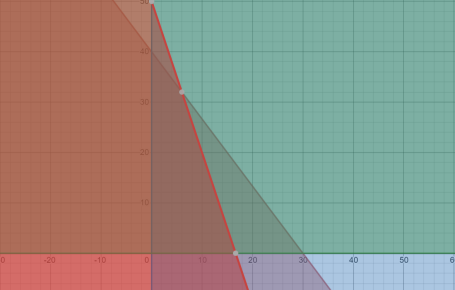
The linear programming is solved using graphical method and the results presented below;
- Combination of cloth and leather handbags to be produced by the firm
The firm will have to produce 40 leather handbags and zero cloth handbags in order to maximize on the profits.
- Graphical representation
The figure below presents the all the constraints, indicating corner solutions and feasible region.
| Regression Statistics | ||||||||
| Multiple R | 0.399132618 | |||||||
| R Square | 0.159306847 | |||||||
| Adjusted R Square | 0.001676881 | |||||||
| Standard Error | 10865.20156 | |||||||
| Observations | 20 | |||||||
| ANOVA | ||||||||
| df | SS | MS | F | Significance F | ||||
| Regression | 3 | 357925375 | 119308458.3 | 1.010638082 | 0.413753505 | |||
| Residual | 16 | 1888841680 | 118052605 | |||||
| Total | 19 | 2246767055 | ||||||
| Coefficients | Standard Error | t Stat | P-value | Lower 95% | Upper 95% | Lower 95.0% | Upper 95.0% | |
| Intercept | 62688 | 4859.065857 | 12.90124519 | 7.15642E-10 | 52387.24054 | 72988.75946 | 52387.24054 | 72988.75946 |
| 1st Qtr | -106 | 6871.756835 | -0.015425459 | 0.987883466 | -14673.47373 | 14461.47373 | -14673.47373 | 14461.47373 |
| 2nd Qtr | 2612 | 6871.756835 | 0.380106582 | 0.708864772 | -11955.47373 | 17179.47373 | -11955.47373 | 17179.47373 |
| 3rd Qtr | 10276 | 6871.756835 | 1.495396337 | 0.154273268 | -4291.47373 | 24843.47373 | -4291.47373 | 24843.47373 |
| regression equation Y=62688-106b1+2612B2+10276B3+e | ||
| regression equation Y=62688-106b1+2612B2+10276B3+e | yrs 1 1st quarter lumber demand=62688-106=62582 | |
| yrs 1 1st quarter lumber demand=62688-106=62582 | yrs1 2nd quarter lumber demand=62688+2612=65300 | |
| RESIDUAL OUTPUT | yrs1 3rd quarter lumber demand=62688+10276=72964 | |
| yrs 1 4th quarter demand =62688 | ||
| Observation | Predicted US Lumber demand | Residuals |
| 1 | 62582 | -16442 |
| 2 | 65300 | -14840 |
| 3 | 72964 | -15344 |
| 4 | 62688 | -14068 |
| 5 | 62582 | -5102 |
| 6 | 65300 | -5850 |
| 7 | 72964 | -6274 |
| 8 | 62688 | -6808 |
| 9 | 62582 | -52 |
| 10 | 65300 | 2140 |
| 11 | 72964 | 1306 |
| 12 | 62688 | 3072 |
| 13 | 62582 | 9298 |
| 14 | 65300 | 6820 |
| 15 | 72964 | 7966 |
| 16 | 62688 | 7022 |
| 17 | 62582 | 12298 |
| 18 | 65300 | 11730 |
| 19 | 72964 | 12346 |
| 20 | 62688 | 10782 |