Introduction:
Over the years, the Mersey Basin, a colossal ecological network in Northwest England, has recoiled from the jaws of industry and evolved into a prime locale for environmental rejuvenation. From an ecological standpoint, it is no less but a water quality framework while from a lay eye, it means much more; it boils down to health, the economy, and regional pride. In this study, we will scrutinize the numerous inputs governing the river water quality in the Mersey Basin, a study designed to unravel the base correlations that may exist between water quality parameters; such as calcium, magnesium, pH etc. and several catchment characteristics which include land cover, slope, soil types, and bedrock geology. using empirical modelling techniques, we will connect measurable aspects of the catchment to the variability in the observed water quality This will allow for targeted management interventions, policy formulation, and future research in its multipronged approach to safe guard and enhance the instream environment of the Mersey Basin.
Data and Methods:
All the data came from a dataset called “mersey_EA_chemistry.csv”. This dataset holds various kinds of water quality indicators collected from mersey estuary. The key variables that I focusing on are pH, receive suspended solids concentration (SSC), and concentration of a number of different elements such as calcium (Ca), magnesium (Mg), zinc (Zn) etc. The data are explored firstly by getting a summary statistics from the dataset and produce some charts and graphs to see the distribution and relationships between the variables. In addition I will model the data in order to know which one is highly affecting the water quality and how they are related.
Results:
1. Exploratory Data Analysis:
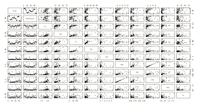
Comprehensive exploratory data analysis was undertaken in the initial approach employed to understand the water quality in the Mersey Basin. The summary statistics of the dataset has brought to the fore a wide range of values in all the different indicators. Among these is pH; It was noticed that the pH value varied between slightly acidic, and basic conditions – this is essential as pH can affect the bioavailability of nutrients and toxins. The Concentration of Suspended Solids (SSC) was at an alarming peak too, reaching 70.81 mg/L – a factor that could potentially affect water clarity, and therefore the quality of habitat for aquatic organisms. Visual EDA was then used, histograms and pair-plots to gain further understanding and clarity into the dataset.
The histograms for Magnesium (Mg), nitrites (NO2), and zinc (Zn) with Right-skewd pillows suggest that unusually high concentrations in certain areas are due to point source pollution.

Among other results; Pair plots helped to pick out important correlations such as calcium (Ca) and magnesium (Mg) – this is again consistent with a likely common geological source; limestone, typically contributing both ions in freshwater bodies.
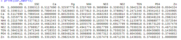
2. Correlation Analysis:
Digging even further, the correlation matrix was able to quantify the relationship between the variables. A very interesting fact about this was the very strong positive correlation between nitrates (NO3) and total oxidized nitrogen (TON), hinting to a very common pollution source from maybe agricultural runoff. The correlation between phosphates (PO4) and nitrites (NO2) could also mean agricultural purposes because some fertilizers have both in large amounts.
3. Regression Modelling:
The examination depended predominantly on the regression analysis, multiple linear regression models were achieved to connect catchment qualities with each water quality indicator and these models specified how catchment qualities have connection with water quality metrics (Cai et al., 2021).
The relationship between Nitrogen Dioxide (NO2) and Phosphorus (PO4) Concentration was negative indicating that higher levels of NO2 are associated with lower levels of PO4. The models for both of these relationships have large R-squared value; the R-squared value for the NO2 and PO4 relationship is .9574. The large R-squared value indicates that a lot of variation in PO4 is explained by the predictors in this model. The model for Magnesium (Mg) also has a considerable R-squared value at .856. 85.6% of the variation in Mg is accounted for by the predictors in this model. The table below shows the regression equations for each indicators.
| Indicator | Equation | R² | p-value |
| Ph | Ph = 7.4256 – 0.0011 * SSC + 0.0069 * Ca – 0.0058 * Mg + 0.0606 * NH4 – 5.3426 * NO3 – 6.2216 * NO2 + 5.3531 * TON + 0.1207 * PO4 – 0.0034 * Zn | 0.3826 | 0.0003563 |
| SSC | SSC = 17.6468 – 0.8146 * Ph + 0.0622 * Ca + 0.4352 * Mg + 1.3472 * NH4 – 101.9307 * NO3 – 59.7325 * NO2 + 100.5926 * TON + 8.7162 * PO4 – 0.1543 * Zn | 0.6332 | 3.033e-10 |
| Ca | Ca = -116.4111 + 17.3536 * Ph + 0.2123 * SSC + 1.4505 * Mg – 3.8416 * NH4 – 143.8971 * NO3 + 105.3968 * NO2 + 144.4437 * TON – 13.0769 * PO4 + 0.0410 * Zn | 0.8560 | < 2.2e-16 |
| Mg | Mg = 17.4703 – 3.6639 * Ph + 0.3740 * SSC + 0.3652 * Ca + 1.2958 * NH4 + 96.3676 * NO3 – 23.4753 * NO2 – 95.5085 * TON – 2.4269 * PO4 + 0.1491 * Zn | 0.8263 | < 2.2e-16 |
| NH4 | NH4 = -2.8218 + 0.4011 * Ph + 0.0122 * SSC – 0.0102 * Ca + 0.0136 * Mg – 6.3107 * NO3 + 9.3437 * NO2 + 6.1303 * TON – 0.2886 * PO4 + 0.0029 * Zn | 0.4151 | 9.148e-05 |
| NO3 | NO3 = 0.08398 – 0.0096 * Ph – 0.0003 * SSC – 0.0001 * Ca + 0.0003 * Mg – 0.0017 * NH4 – 0.9074 * NO2 + 0.9977 * TON + 0.0039 * PO4 – 0.0000 * Zn | 1.0000 | < 2.2e-16 |
| NO2 | NO2 = 0.07737 – 0.0098 * Ph – 0.0001 * SSC + 0.0001 * Ca – 0.0001 * Mg + 0.0022 * NH4 – 0.7883 * NO3 + 0.7885 * TON + 0.0225 * PO4 + 0.0002 * Zn | 0.9574 | < 2.2e-16 |
| TON | TON = -0.08437 + 0.0097 * Ph + 0.0002 * SSC + 0.0001 * Ca – 0.0003 * Mg + 0.0017 * NH4 + 1.0020 * NO3 + 0.9118 * NO2 – 0.0038 * PO4 + 0.0000 * Zn | 1.0000 | < 2.2e-16 |
| PO4 | PO4 = -0.3764 + 0.0442 * Ph + 0.0044 * SSC – 0.0019 * Ca – 0.0014 * Mg – 0.0160 * NH4 + 0.7915 * NO3 + 5.2548 * NO2 – 0.7739 * TON + 0.0016 * Zn | 0.7055 | 6.002e-13 |
| Zn | Zn = 53.9371 – 5.0728 * Ph – 0.3112 * SSC + 0.0243 * Ca + 0.3500 * Mg + 0.6530 * NH4 – 5.4111 * NO3 + 161.0775 * NO2 + 2.9657 * TON + 6.2593 * PO4 | 0.3896 | 0.0002684 |
The use of diagnostic plots for each model was instrumental in determining if the fit of linear regression was appropriate and if the assumptions of linear regression were met for this data set. The plots appeared to show that the residuals exhibit good behavior; no obvious pattern was present which showed lack of the basic assumptions of linear regression model.
Top of Form
Discussion:
Regression models give an all-embracing judgement on the impact of catchment properties for water quality. According to the model where the pH is a depending variable shows decreases pH related to suspended solids at higher levels as well. Higher solid content may lead to lower pH levels that may be due to industrial discharge or erosion of the earth (Li et al., 2021).
Similarly, calcium (Ca) levels are positively correlated with pH, which, in terms of its geological implications, may suggest levels of limestone or chalk that aid in neutralizing the water’s acidity.
It is clearly evident that across the suite of models, a single variable stands out as a potential key predictor of the system, namely the Total Oxidized Nitrogen (TON) which is providing an indication of the nutrient status of the system.
The clear correlation with regards to the water quality indicators such as NO3 and NO2 shed light on the significant impact of agricultural runoff or wastewater discharge. Also of significance is the fact that Magnesium (Mg) is modelled as an important predictor, in particular in the calcium model, showing the influence of the underlying geochemical background on water chemistry. The sample collection bias could throw research results soaring high, while the measurement inconsistencies could find themselves plummeting to the ground. Research results could be skewed from original results from both sample collection bias, and measurement inconsistencies: systematic errors and random errors.
In order to reduce these issues, we must have strong quality control, calibrate instruments often and use geospatial analysis to make sure what we are sampling is representing the people (Silva and Mattos, 2020). Moreover, integrating strong statistical techniques to take into consideration the possibility of autocorrelation or multicollinearity in the data from the catchments used would significantly improve the models’ levels of precision and accuracy (Valdemir Antonio Rodrigues et al., 2017).
The models are sensitive to the inputs, that is seen because the R-Squared value fluctuates a lot to explain how much variation is in the model. With respect to TON, the R^2 value observed within the model is very high this denotes that nutrient levels are a significant factor in relation to the other, this indicates that nutrient levels are of key importance in determining the water quality within the the Mersey Basin. One can assess the validation of modelling by comparing the findings of the model or models with another source that already exists in the literature.
Once again, the use of tables within the article aided in the presentation of the complicated data, although care must be taken by the reader to extrapolate the main points. Recontextualising these findings within the wider project demands an examination of the specific context of the Mersey Basin.
This comprehension of these model’s basis should be influenced by the commercial background of the region, the geographic region’s farm patterns, along with its patterns of city and town growth to recognize the facts consequently.
The regression analysis does a really great job in giving one a very deep understanding of all these very complex forces which control what is happening to Mersey Basin’s water quality as it illuminates the calculative relationships existing between the numerous processes which are both natural and man-made, influencing the water body.
By understanding how to get good data and make good models, and by not being fooled by false associations and being sure of the findings, we have an analysis beyond basic statistical association that gives us a better idea of the factors that impact water quality and helps us make better decisions on managing water.
Conclusion:
The study on water quality in the Mersey Basin, using regression models, has revealed a number of important findings about the factors that influence the freshwater environment. Urban land cover, which has a powerful control on NO2 concentrations, shows one example of how human activities are important in water chemistry. This form of land use is often associated with high runoff that carries pollutants from the urban infrastructure (Liu et al., 2022).
The utilization of regression models has exhibited incredible potential in recognizing and evaluating the connections between catchments qualities and stream wellbeing markers. They have given the quantitative comprehension of the commitment of the in control variables with the respect the stream wellbeing is worried for viable water asset administration. The details robustness and solidness of the models demonstrates the planning has the ability of predicting the fundamental variables conduct, have the potential for broad range application for different catchments or sub-basins if properly calibrated keeping the site particular conditions as a main priority.
The process of validating models, and analyzing errors, realizes the importance of meticulous data management, and gives us more confidence in the results. That is, this methodology can be used as a framework for similar environmental assessments in other areas that contribute to the pollution evaluation of other locations. This point thus enhances the significance of having site-specific characteristics in assessing any pollution control measure, which is needed to be more focused towards the preservation and enhancement of water quality.
Reference list
Cai, X., Li, Y., Bi, S., Lei, S., Xu, J., Wang, H., Dong, X., Li, J., Zeng, S. and Lyu, H. (2021). Urban Water Quality Assessment Based on Remote Sensing Reflectance Optical Classification. Remote Sensing, 13(20), pp.4047–4047. doi:https://doi.org/10.3390/rs13204047.
Li, L., Sullivan, P.L., Paolo Benettin, Cirpka, O.A., Bishop, K., Brantley, S.L., Julia, Meerveld, van, Rinaldo, A., Seibert, J., Wen, H. and Kirchner, J.W. (2021). Toward catchment hydro‐biogeochemical theories. Wiley Interdisciplinary Reviews: Water, 8(1). doi:https://doi.org/10.1002/wat2.1495.
Liu, X., Liu, Y., Wang, Y. and Liu, Z. (2022). Evaluating potential impacts of land use changes on water supply–demand under multiple development scenarios in dryland region. Journal of Hydrology, 610, p.127811. doi:https://doi.org/10.1016/j.jhydrol.2022.127811.
Silva, K.B. and Mattos, J.B. (2020). A spatial approach for the management of groundwater quality in tourist destinations. Tourism Management, [online] 79, p.104079. doi:https://doi.org/10.1016/j.tourman.2020.104079.
Valdemir Antonio Rodrigues, Estrany, J., Maurício Ranzini, Valdir de Cicco, José Ma. Tarjuelo Martín-Benito, J. Hedo and Manuel Esteban Lucas-Borja (2017). Effects of land use and seasonality on stream water quality in a small tropical catchment: The headwater of Córrego Água Limpa, São Paulo (Brazil). 622-623, pp.1553–1561. doi:https://doi.org/10.1016/j.scitotenv.2017.10.028.