Introduction
Air pollution remains one of the major public health hazards in urban areas of developing nations where rapid urbanization and growth of industries often outreach the capacity of environmental regulative framework. Traffic-related pollution, more precisely vehicle-generated emissions, very significantly contributes to poor air quality, which worsens respiratory and cardiac conditions among the citizens in cities. Precisely, this paper seeks to investigate variations of different physical features at urban road intersections with a view to determine the concentration of airborne pollutants such as CO, PM2.5, and PM10.
Previous studies have identified traffic flow, road width, and the presence of stoplights as pertinent variables in predicting pollutant levels. However, how these variables interact within the urban environment of a developing nation has not been adequately represented with data. Data for this study were collected at 30 intersections within a large city. It will serve to provide actionable insight that can be of importance in guiding urban planners and policy makers to take steps aimed at reducing the traffic-related air pollution problem, thus improving the health outcomes for the public.
Literature Review
The contribution of traffic-related pollution to urban air quality has been well documented principally in developed countries with stringent environmental measures in place. However, the fast-rising literature on developing nations, where rapid urbanization and motorization are coupled with huge increments in pollution, is voluminous. This section reviews relevant studies that look at the effects of traffic flow, road configuration, and regimes of traffic management on air quality.
Traffic Flow and Air Pollution: Most of these pollutants, related to traffic flow, have been highly linked to pollutant levels in many studies, including Carbon Monoxide, Nitrogen Oxides, particulate matter, among others. For instance, Apte et al. [1] prove that increased vehicle volume along city roads brings about higher PM2.5 and CO concentrations, with aggravated respiratory and cardiovascular health problems in people near major roadways. These findings are representative of all urban settings and, to some extent, show just how critical traffic flow is in determining air quality.
Road Infrastructure: In this respect, the role of width and infrastructure of a road has been greatly looked into as influencing factors of pollution. Wider roads allow better dispersion, hence a reduced concentration at ground level. According to Su et al. [2], narrow and densely populated urban areas contribute to accumulation due to limited circulation of air, mainly PM10. Therefore, this shows that design and urban planning are critical in mitigating pollution.
Traffic Management Strategies: These traffic management strategies, including optimal timing of traffic signals and congestion pricing, have been very effective ways to reduce emissions and improve air quality. For example, Kwak [3] showed how the optimal timing of traffic signals can minimize time spent idling at intersections, reducing CO emission and associated pollutants. These policies are extremely relevant for developing nations where traffic congestion is one of the main contributors to poor air quality.
This literature review underlines the proper understanding of the traffic flow, road infrastructure, and its traffic management interplay in mitigating urban air pollution. The insights obtained from these studies have guided the current study, which was conducted with the view of applying these concepts within an urban environment in a developing nation.
Methodology
Data Collection
The dataset used in this study consists of measurements from 30 intersections in a large city in a developing country. Measurements used in this study include CO, PM2.5, PM10, and each datum is the mean pollutant concentration over a period of 15 minutes for three distinct periods of the day: early morning, morning rush, evening rush.
Besides pollutant levels, there are a large group of site characteristics in this dataset which may be affecting, or related to, air quality. Those can be grouped into two separate groups: variables that are dynamic (change depending on the time of the day), like traffic flow and vehicle count, and variables that are static, such as road width and presence of stoplights.
Data Preprocessing
Cleaning of the dataset was done in the preprocessing step itself by replacing missing values and condensing categorical variables into a format suitable for analysis. Again, in case of missing values for every variable in data Integrity, the median value for that variable is imputed to replace the NaN values. Categorical variables such as median or stoplight were converted into binary indicators.
# Drop irrelevant columns and columns that are not needed for the model
data_df = data_df.drop(columns=[‘Unnamed: 29’, ‘Date’, ‘Time’])
# Replace missing values represented by ‘.’ with NaN
data_df.replace(‘.’, np.nan, inplace=True)
# Convert categorical variables to categorical data types
categorical_cols = [‘Median’, ‘Stop_traffic’, ‘Traffic_flow’, ‘Upwind_source’, ‘Hill’, ‘Hill_near’]
data_df[categorical_cols] = data_df[categorical_cols].astype(‘category’)
# Separate numerical & categorical columns
numeric_cols = data_df.select_dtypes(include=[np.number]).columns
categorical_cols = data_df.select_dtypes(include=[‘category’]).columns
# Impute missing values
numeric_imputer = SimpleImputer(strategy=’median’)
data_df[numeric_cols] = numeric_imputer.fit_transform(data_df[numeric_cols])
categorical_imputer = SimpleImputer(strategy=’most_frequent’)
data_df[categorical_cols] = categorical_imputer.fit_transform(data_df[categorical_cols])
# Verify that there are no remaining NaN values
print(“Missing values in the dataset after cleaning:”)
print(data_df.isnull().sum().sum())
3.3 Exploratory Data Analysis (EDA)
Exploratory Data Analysis was conducted to understand distribution and relationships in the dataset. Descriptive statistics measures were computed for the indicators of primary pollutants, along with histograms to see their distribution. Also, the correlation matrix was developed to check relationships between site variables and pollutant concentrations.
# Summary statistics for the primary pollutants of interest
pollutants = [‘PM2.5_AVG’, ‘PM10_AVG’, ‘CO_AVG’]
summary_stats = data_df[pollutants].describe()
summary_stats
# Visualize the distribution of each pollutant using histograms
sns.set(style=”whitegrid”)
for pollutant in pollutants:
plt.figure(figsize=(10, 6))
sns.histplot(data_df[pollutant], kde=True, bins=15, color=’blue’)
plt.title(f’Distribution of {pollutant}’)
plt.xlabel(f'{pollutant} Concentration’)
plt.ylabel(‘Frequency’)
plt.show()
# Correlation matrix (excluding ‘Time’ due to blank values)
corr_matrix = data_df.drop(columns=[‘Time’]).corr()
plt.figure(figsize=(20, 15))
sns.heatmap(corr_matrix, annot=True, fmt=’.2f’, cmap=’coolwarm’, linewidths=0.5)
plt.title(‘Correlation Matrix of All Variables’)
plt.show()
Statistical Modeling
A linear model was applied to the interrelation of site characteristic variables with pollutant concentration variables in the data set. This was performed by running 70–30 of the dataset division into both training and test datasets. The model’s efficiency needed to be evaluated using such metrics as Mean Squared Error (MSE) and R-squared (R²).
# Splitting data into features (X) and target (Y) for modeling
pollutants = [‘PM2.5_AVG’, ‘PM10_AVG’, ‘CO_AVG’]
X = data_df.drop(columns=pollutants)
Y = data_df[pollutants]
# Splitting the data
X_train, X_test, Y_train, Y_test = train_test_split(X, Y, test_size=0.3, random_state=42)
# Initializing the model
model = LinearRegression()
# Fitting the model
model.fit(X_train, Y_train)
# Predictions
Y_pred = model.predict(X_test)
# Evaluating the model
mse = mean_squared_error(Y_test, Y_pred)
r2 = r2_score(Y_test, Y_pred)
mse, r2
Results
Summary Statistics
The summary statistics of the main pollutants of CO, PM2.5, and PM10 showed rather significant changes in pollutant concentrations at the various times of the day. Generally, higher PM2.5 concentrations were experienced during the morning rush hour periods, while CO peaked in the evening rush. However, there is less variation in the levels of PM10 conclusively among the different periods.
Visualizations of Pollutant Distributions
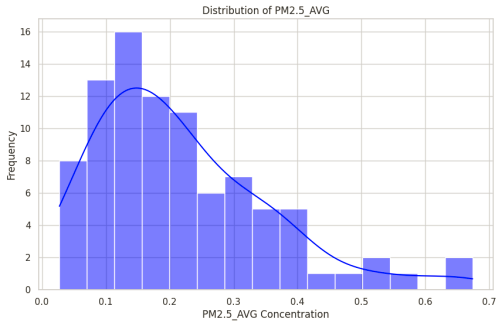
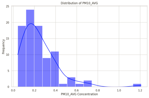
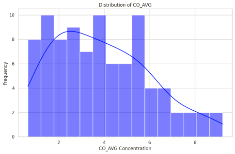
Histograms of pollutant distributions were plotted to image the spread and central tendency of the data. All plots showed a skewed distribution in pollutant concentrations, with higher frequencies of lower concentrations and a long tail extending toward higher values.
PM2.5 Distribution: The histogram of PM2.5_AVG shows a right-skewed distribution where most values are at 0.1 to 0.3, although outliers reach as high as 0.67.
PM10 Distribution: The histogram to the variable PM10_AVG also forms a right-skew distribution with values mainly lying between 0.1 and 0.4, with outliers extending up to 1.2
CO Distribution: CO_AVG has a smaller skew, still slightly higher in concentration, then tapers off with a long tail up to 9.2 ppm.
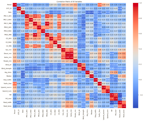
Correlation Analysis
The correlation matrix evidenced several strong relationships in site characteristics with pollutant concentrations. For instance, there was an obvious positive correlation between traffic flow with levels of PM2.5 and CO, which illustrates that higher vehicular volume might lead to a larger number of pollutants. The presence of stoplights was also related to higher concentrations of CO due to probable idling at an intersection
Regression Model Results
Linear regression was done to relate site characteristics to pollutant concentrations. Evaluation metrics after cleaning the dataset and conducting model training turned in:
Mean Squared Error (MSE): 0.469
R-squared (R²): 0.580
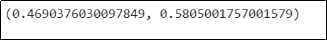
These results indicate that about 58% of the variance in pollutant concentrations is explained by the model, so it has quite a moderate fit. While this model does pick up part of the relationship between variables, there may well be other factors at play in pollutant levels not being modeled.
Model Coefficients
The coefficients from the regression model showed the magnitude and direction of the relationships between site characteristics and pollutant concentrations. In this case, increases in road width were associated with reductions in PM10 while greater traffic flow was related to increased CO. These findings may be expected, as wider roads might allow for greater dispersion of pollutants, and greater volumes of traffic generally translate into more emissions.

Discussion
Interpretation of Results
Results in this study support the available literature, which describes the role of traffic and site characteristics in the variation of air quality. The strong positive association of traffic flow in conjunction with levels of the pollutants shows the importance of enforcing sound traffic management practices to reduce pollution, especially in heavily urbanized and populated areas. The identification of the stoplight as a statistically independent contributor to higher CO showed traffic signal timing practices as a potential public health edge with minimization of idle time for vehicles, which contributes to lower air pollution.
Implications for Urban Planning
From this overview, important implications for urban planning can be realized. That is, the policymakers would better place themselves to target areas for intervention after identifying the factors influencing urban air quality most strongly. By way of an example, the infrastructure at intersections with high traffic volume and narrow roads could get better: road-widening, or even better, the setting up of a traffic management system. It further highlights that green infrastructure can assist in absorbing and scattering pollutants by integrating medians and green belts into spaces.
Limitations and Future Research
While this study is very insightful, there exist some important limitations that must be duly identified. First, the dataset comprised only 30 intersections within one city, which inherently limits generalizability. Second, there are site-specific features other than those considered here that can influence the level of pollutants, such as weather conditions and nearby industrial activities. Future studies could further this research by sampling more intersections from multiple cities.
Conclusion
The current research has sought to establish the nature of the relationships among various site characteristics and traffic-related air pollution within an urban environment in a developing country. This study used linear regression modeling in order to find important predictor variables of pollutant concentrations, including traffic flow, road width, and stoplights. The findings provide actionable insight: targeted intervention can be effective for mitigating air pollution in highly urban areas, through optimizing traffic flows or widening the roads.
These results from the study underline the importance of site considerations in any strategy to abate traffic pollution. Correlation and regression analyses showed variations of the impact of site characteristics on pollutant levels under certain conditions, such as time of day and urban context. This confirms the need for a type of solution that is situation-based and takes into account the individual features of each particular site.
The present research thus contributes to the growing body of literature centered on urban air quality and provides pragmatic recommendations toward the enhancement of air quality in cities, particularly developing countries. In summary, the key findings suggest that planning and traffic management at the urban level need to be incorporated as intrinsic components of policies targeted at reducing air pollution. While this study forms the strong base for further works with respect to this theme, more studies are required in order to support findings in different urban contexts and to deepen the investigation of other variables that might influence pollution at those measurement locations, relating to meteorological conditions and industrial activities.
References
J. S. Apte, M. Brauer, A. J. Cohen, M. Ezzati, and C. A. Pope, “Ambient PM2.5 Reduces Global and Regional Life Expectancy,” Environmental Science & Technology Letters, vol. 5, no. 9, pp. 546–551, Aug. 2018, doi: https://doi.org/10.1021/acs.estlett.8b00360.
J. G. Su, M. Jerrett, B. Beckerman, M. Wilhelm, J. K. Ghosh, and B. Ritz, “Predicting traffic-related air pollution in Los Angeles using a distance decay regression selection strategy,” Environmental Research, vol. 109, no. 6, pp. 657–670, Aug. 2009, doi: https://doi.org/10.1016/j.envres.2009.06.001.
Kwak, B. Park, and J. Lee, “Evaluating the impacts of urban corridor traffic signal optimization on vehicle emissions and fuel consumption,” Transportation Planning and Technology, vol. 35, no. 2, pp. 145–160, Mar. 2012, doi: https://doi.org/10.1080/03081060.2011.651877.