Description of the problem
A cylinder of diameter 1 cm is subjected to a uniform flow, whose free-stream velocity us U. The aim is to analyse the aerodynamic behaviour of the flow at different Reynolds numbers (Re), that is, at Re = 1, Re = 25, Re = 75, and Re = 150. CFD (Computational Fluid Dynamics) analysis is to be performed for each Reynolds number and iso-contours of pressure and velocity, vector plots of velocity for different Reynolds number is to be plotted.
Numerical Method
Since the simulation is focused on the external aerodynamics of the model and the compressibility effects in the flow are not relatively dominant, ‘pressure-based’ solver, with ‘2D planar’, and ‘transient’ (unsteady) solver options were chosen to solve the problem. The viscous model is chosen to be ‘laminar’. The fluid is water; having a constant density of 1000 kg/m3 and a viscosity of 0.001 kg/m-s.
A tetrahedral mesh is created in the fluid domain. The mesh near the 2D cylinder is much denser than the mesh at the other boundaries. The boundary at the extreme left is given as the ‘inlet’, where the velocity corresponding with the Reynolds number is given as the input. The value of the velocity is obtained from the equation:
U =
Where,
Re – is the Reynolds number
µ – viscosity (for water, the value of µ = 0.001 kg/m-s)
D – diameter of the cylinder (in m) = 1 x 10⁻² m
ρ – density of water = 1000 kg/m3
U – velocity of fluid (in m/s)
Using the above equation, the values of velocities with the corresponding Reynolds number is obtained to be:
| Reynolds Number | Velocity (in m/s) |
| 1 | 1 x 10⁻⁴ |
| 25 | 2.5 x 10⁻³ |
| 75 | 7.5 x 10⁻³ |
| 150 | 0.015 |
PISO (Pressure-Implicit with Splitting of Operators) scheme of solution method is chosen to solve the problem. This type of solution method allows to solve or obtain the solution of the problem with a mesh having high skewness (ANSYS 2019). The skewness correction is given as 1 and the neighbour correction is given as 1 (Miau et al. 2014).
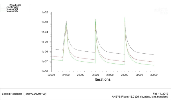
The residuals of the continuity equation are kept smaller (1 x 10-16) to obtain high accuracy in the results (Li & Wood 2018). The solution is then initialized using the ‘standard’ method of initialization.
The time-steps used for different cases are listed below:
| Reynolds Number | Time Step | Number of Iterations per Time Step |
| 1 | 0.8 | 2000 |
| 25 | 0.5 | 2000 |
| 75 | 0.3 | 2000 |
| 150 | 0.2 | 200 |
Results
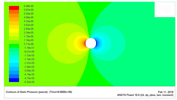
Figure 1: Typical Residuals Plot
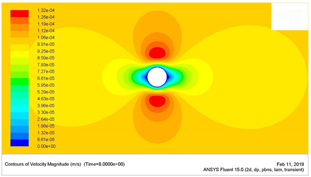
Figure 2: Static Pressure Contours for Re = 1
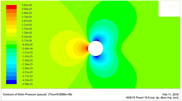
Figure 3: Velocity Contours for Re = 1
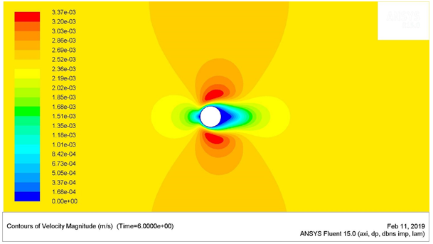
Figure 4: Static Pressure Contours for Re = 25
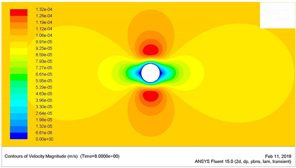
Figure 5: Velocity Contours for Re = 25
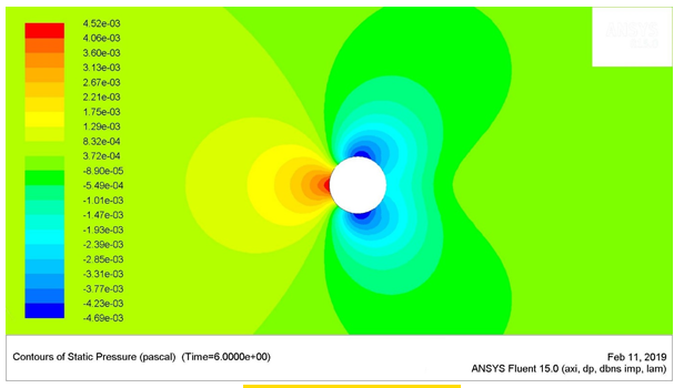
Figure 6: Static Pressure Contours for Re = 75
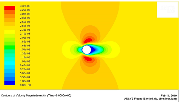
Figure 7: Velocity Contours for Re = 75
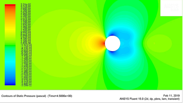
Figure 8: Static Pressure Contours for Re = 150

Figure 9: Static Pressure Contours for Re = 150
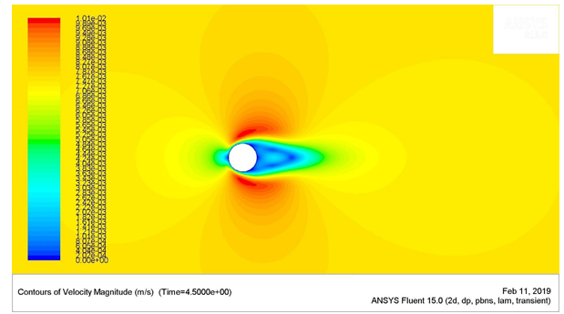
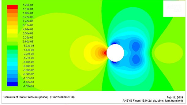
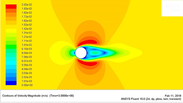
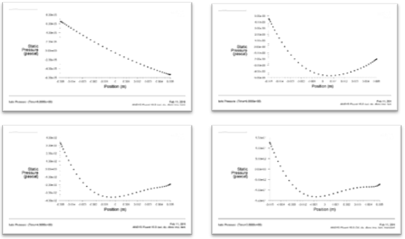
Figure 10: Static Pressure around the cylinder at Re = 1 (top left), Re = 25 (top right), Re = 75 (bottom-left), and Re = 150 (bottom-right)
The following is the results of the coefficient of drag of the given cylinder for different Reynolds number.
| Reynolds Number | Coefficient of Drag |
| 1 | 0.3374 |
| 25 | 0.0223 |
| 75 | 0.01842 |
| 150 | 0.00125 |
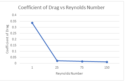
Figure 11: Plot of CD vs Re
Flow patterns as a function of the Reynolds number:
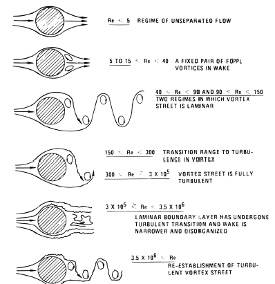
Figure 12: Various types of flow around a circular cylinder in relation with Reynolds Number
For the lower Mach numbers, the flow remains attached to the geometry of the cylinder and it remains almost symmetric about the horizontal symmetrical axis of the cylinder. For the Reynolds number between 4 and 40, the flow starts to detach at the far end of the cylinder or at the back of the cylinder. This flow forms two distinct vortices near the cylinder. As the Reynolds number is increased above 40, the flow becomes unstable. However, the flow pattern shows a regular wake in the downstream of the flow (Anderson 2016).
When the Reynolds number is further increased, say, from 1000 to 3 million (3 x10⁵), the flow starts to become turbulent. The flow separation is now near the 80 ͦ from the stagnation point. The wake is comparatively longer. Beyond the Reynolds number of 3 million, the turbulent intensity increases and the flow starts to attach and separate near 120 ͦ from the stagnation point.
Hydrodynamic forces: effect of Reynolds number:
The drag coefficient (Cd) can be obtained by the equation:
Cd = –
Where,
Cp is the coefficient of pressure at different points (in terms of angles) around the cylinder. This integration can be done numerically using Simpson’s rule.
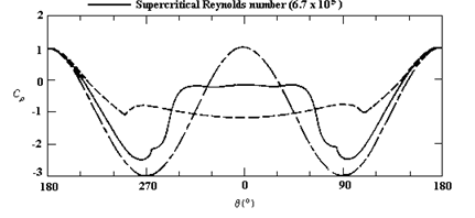
Figure 13: Typical Pressure distributions on a circular cylinder in relation with Reynolds number (Verzicco et al. 2010)
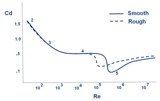
Figure 14: Typical Theoretical Plot of Coefficient of Drag of Circular Cylinder (of the smooth and rough surface) with Reynolds Number (NASA 2015)
Summary and Discussion
CFD analysis for the flow over circular cylinder is done for different low Reynolds numbers. The iso-contour plots of the pressure and velocity have been addressed in the figures (2), (3), (4), (5), (6), (7), (8), and (9).
The maximum stagnation pressure for the Reynolds number of 1 was found to be 6.459 e-5 Pa, which was located at the stagnation point (the very left-most point) of the circular cylinder. The minimum stagnation pressure was found to be -5.3175 e-5 Pa, which was located just behind the circular cylinder.
The maximum stagnation pressure for the Reynolds number of 25 was found to be 45.16 e-4 Pa, which was located at the stagnation point (the very left-most point) of the circular cylinder. The minimum stagnation pressure was found to be -46.94 e-4 Pa, which was located near the angle 120 ͦ and 210 ͦ , measured in the clockwise direction from the stagnation point of the cylinder.
The maximum stagnation pressure for the Reynolds number of 75 was found to be 0.03307 Pa, which was located at the stagnation point (the very left-most point) of the circular cylinder. The minimum stagnation pressure was found to be -0.03582 Pa, which was located near the angle 80 ͦ and 280 ͦ , measured in the clockwise direction from the stagnation point of the cylinder.
The maximum stagnation pressure for the Reynolds number of 75 was found to be 0.12594 Pa, which was located at the stagnation point (the very left-most point) of the circular cylinder. The minimum stagnation pressure was found to be -0.132508 Pa, which was located near the angle 65 ͦ and 295 ͦ , measured in the clockwise direction from the stagnation point of the cylinder.
The shear stresses were higher near the regions of flow separation. These regions have been highlighted in the above points, where the stagnation pressure was the lowest. The up-down symmetric behaviour of the flow was observed for the Reynolds numbers 1 and 25. The length of the wake gradually increased with the increase in the flow velocity or Reynolds number.
The effect of the drag force in relation to the Reynolds number is shown in the figure-11. The lower Reynolds numbers gave comparatively higher drag coefficients. This behaviour of the flow was closely matched with the theoretical results from figure -14. The relation of the drag is directly proportional to the square of the velocity of the fluid. In case the velocity of the flow is doubled, the drag will be quadrupled. Similarly, the Reynolds number has almost linear relationship with the velocity of the flow. It is directly proportional to the velocity of the fluid. On the other hand, the pressure is inversely proportional to the Reynolds number. As the Reynolds number increases, the velocity of the flow will increase and where there is an increase in the velocity, there will be decrease in the pressure.
If there was more time available to work on this assignment, more accurate CFD results could have been performed. The time step size of 0.01 can be used for over 20 or 30 time-steps with 2000 iterations per time step. The mesh can be denser while maintaining appropriate y-plus value for the mesh for the corresponding turbulence model. The CFD analysis can also be performed for higher Reynolds numbers as well and the results can be compared with the available theoretical results. Also, the analysis can also be focused on the wake produced by the circular cylinder, like- the length of the wake, the pattern produced by the flow past the cylinder, and vortex shedding.
References
Anderson, J.D. 2016, Fundamentals of Aerodynamics. Mcgraw – Hill Education, New York.
ANSYS. 2019, Choosing the Pressure-Velocity Coupling Method, viewed 11 February 2019, <https://www.sharcnet.ca/Software/Fluent6/html/ug/node1021.htm>
Li, Z. and Wood, R. 2018, ‘CFD Analysis of 2D Unsteady Flow Past a Square Cylinder at Low Reynolds Numbers’, ITM Web of Conferences, viewed 11 February 2019, <https://www.itm-conferences.org/articles/itmconf/abs/2018/01/itmconf_amcse2018_02003/itmconf_amcse2018_02003.html>
Miau, J., Fang, C., Chen M., and Lai, Y. 2014, ‘Discrete Transition of Flow Over a Circular Cylinder at Pre-critical Reynolds Numbers’, National Cheng-Kung University Publications, viewed 11 February 2019, <https://doi.org/10.2514/1.J052909>
NASA 2015, Drag of a Sphere, viewed 11 February 2019 <https://www.grc.nasa.gov/www/K-12/airplane/dragsphere.html>
Shyy, W. 2011, Aerodynamics of low Reynolds number flyers, 2nd edn, Cambridge University press, Cambridge.
Verzicco, R., Yusof, J., Orlandi, P., and Haworth, D. 2010, ‘Large Eddy Simulation in Complex Geometric Configurations Using Boundary Body Forces’, The American Institute of Aeronautics and Astronautics, vol. 38, viewed 11 February 2019, <https://doi.org/10.2514/2.1001>