Self Check Assignment: Milligan-2375411

Welcome to your hands-on activity! This assignment invites you to work with Tableau using a mix of generated and real-world data. You will follow these steps:

• Download the attached spreadsheets, and upload those data sets into Tableau. If you need help loading your data sources, refer to the Unit 1 Self Check Assignment: Milligan Chapter 1
• Go through this document, and use Tableau to answer all the questions listed below. Where applicable, paste screenshots into the template below.
• When you are ready, complete the online quiz, which verifies your homework. Use the answers you found in this document to answer the questions.
• When you have completed the online quiz, submit the Word document.
• Remember, you can always ask your instructor for help if needed.
• If you need to adjust the size of your visualizations to match the options in the questions, use the “Format”-> “Cell size” options. For example, “Ctrl+Shift+B” on a Windows computer will make the visualization bigger, and “Ctrl+Up” will make it taller.

This assignment contains 7 datasets and 6 icon files:

1. Pacific West National Park Visitation 2001–2022
2. Monthly Personal Budget (two worksheets: July and August)
3. Video game sales
4. 2022 NYC Restaurant Inspections
5. September 2023 Baltimore City Crime Data
6. University course completion rates
7. University pass rates
8. Icon files:
   1. Biology
   1. Chemistry
   1. Computer Programming
   1. Data Analytics
   1. Math
   1. Physics

Question 1: Bump chart

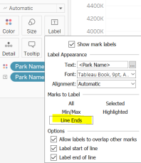
You have been asked to help the Northwest National Park system to find trends. Specifically, what do five-year visitation trends look like for the parks? Load the Pacific West National Park Visitation 2001–2022 into your data sources. Drag “Year” into the columns and create an ad hoc calculation in the row: SUM (Visitor Count). Then drag “Park Type.” Select only the “National Park” park type. Then, drag “Year” into the filters for the years 2018–2022. Keep in mind that the year 2020 will have anomalies due to the COVID-19 pandemic shutdown of many parks. Drag “Park Name” onto “Color” in the “Marks” tab and “Park Name” onto “Label.” Make sure the marks type is set to “Line.” Edit the label so that it shows the “Line Ends.”

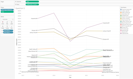
From this chart, we can see that Yosemite, Olympic, and Death Valley all had [missing word], but they took downturns in 2020. They are rising again, but still not seeing the numbers they had previously. Joshua Tree, Mount Rainier, Hawaii Volcanoes, and Haleakala NP have increased visitors in 2022 compared to 2018.

While this is helpful, the leadership has requested to see a chart with 10 years (2013–2022). They also want to see only national parks with at least 1 million visitors annually. Add both filters to your bump chart. Add Visitor Count as a Label.

Question 1A: For the Yosemite NP, was there an increase or decrease between 2013 and 2022?

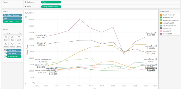
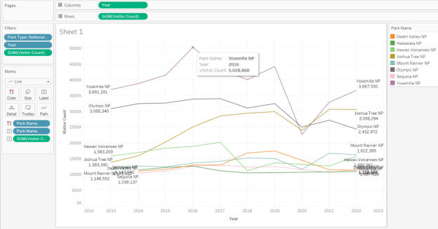
Question 1B: What was the highest visitor count for Yosemite NP between 2013 and 2022?

Question 1B Answer:

It was 5,028,868

Question 2: Waterfall

Your friend is always complaining to you that they can’t save any money and their bank account is always going down. You ask your friend to write down all the expenses and income in a month, and you record them in the Monthly Personal Budget: July. For each expense, you have tracked the date, type, whether it is income, fixed, or discretionary, and the amount (negative for expenses and positive for income).

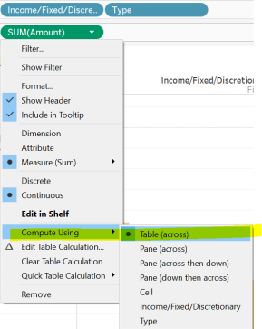
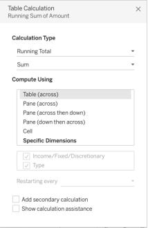
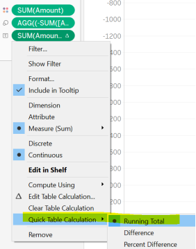
Load the dataset into Tableau and choose the July worksheet to start. Create a waterfall chart of the July data by dragging the “Income/Fixed/Discretionary” and “Type” dimensions into the columns. Then drag “Amount” into the rows. Because we want to see the total as the month goes on, we will create a running total calculation using table across. To do this, first, right-click “Amount” and select “Add Table Calculation…”. This should bring up the following

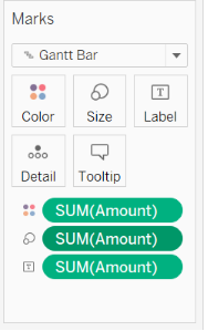
Drag the “Amount” measure onto Color, Size, and Label in the Marks tab.

Change the chart type to “Gantt Bar.”

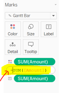
Double-click on “SUM(Amount)” on Size and edit in the shelf. Add a negative sign before the SUM([Amount]).

Change the “SUM(Amount)” on Label to be a Running Total.

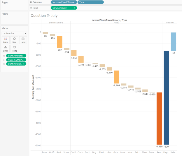
Now, we can see quickly that your friend spent $794 in the month of July just on discretionary spending. Then by the time they paid their rent, they had spent a total of $4,960 for the month. They make $4,140 from their regular job and another $805 from side gigs. This means that in July, your friend overspent their monthly income by $15 dollars. If they spend like that every month, that means they are overspending $180 a year.

Your friend would really like to start saving money, so you help them go through expenses and try to spend less money. Now, they return with their August expenses (another worksheet in the Monthly Personal Budget), and they want to see the same chart.

Question 2: How much money did your friend save this month? Provide your answer rounded to the nearest dollar (no cents).

Question 2 Answer:

<<insert your screenshot>>

Question 3: Step lines

For this exercise, you will be using the “Video game sales” data set to answer questions about how certain genres have performed by global sales in the last five years.

Drag “Genre” over to Columns and “Global Sales” into Rows. Add a quick calculation of Running Total to the “Global Sales.”

Drag “Global Sales” onto Color in the Marks tab.

Filter by Years 2011 to 2016.

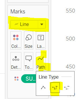
Change the Marks type to “Line,” and then click on “Path” and choose “Step.

Click on Ctrl+Shift+B (or CMD+Shift+B if you’re on a Mac) a few times to make the graph wider (this might help to read the bottom axis better).

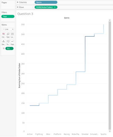
We can see that shooter games had a significant step within global sales between 2011 and 2016.

However, we can see that action starts around $140. Let’s modify this a bit.

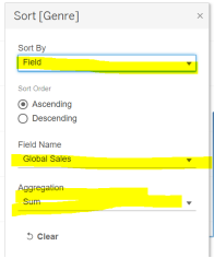
Right-click on “Genre” in the columns area, click on the “Sort” function. We want to sort by Field, Ascending, Field Name-Global Sales, and Aggregation type: Sum.

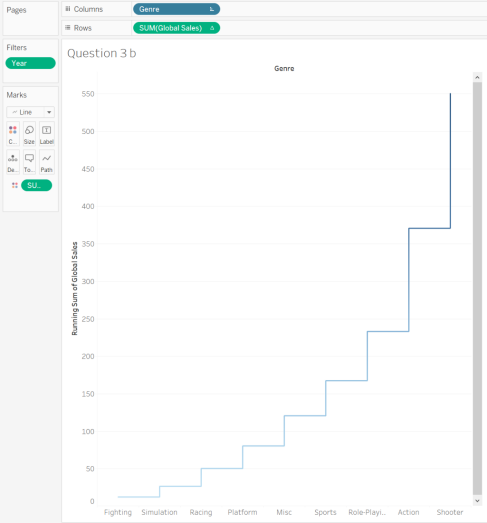
Now, we can see where the calculation starts in the bottom left corner with Fighting and slowly steps up until we get to Action and then Shooter games, where we see two big jumps. This is a better representation of the step-line chart.

Now, change the years to 2006–2010.

Question 3: What is the top-selling genre? What was the amount of global sales for that genre?

Option A: Role-playing, 316.1

Option B: Shooter, 899.3

Option C: Action, 437.4

Option D: Sports, 209.4

Question 3 Answer:

<<insert your screenshot>>

Question 4: Sparklines

You are being asked to find trends about the New York City Health Department Restaurant Inspections. There are over 27,0000 restaurants in the five boroughs of New York City. You need to load the data source: 2022 NYC Restaurant Inspections. This is a rather large data source and may take a little longer to load the data.

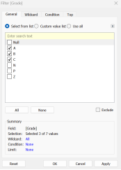
When restaurants have violations, they receive scores for each violation. Therefore, restaurants want low scores, and high scores are not desirable. Grades A–C are assigned to restaurants based on their scores. Restaurants with scores of 0 to 13 receive an “A.” If they score between 14 and 27, they receive a “B.” A “C” grade is 28 or more. If you would like to read more, see ABCEats-Restaurants.

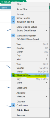
Drag “Inspection Date” into columns and “Boro” into rows. Now pull “Score” into the row, and change the aggregation to “Average” instead of sum. Change the date from ”Year” to ”Week Number” (right-click on the inspection date field in columns).

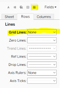
Right-click in the line graph area, and click on format. Then click on the Lines icon, and turn off the gridlines.

Widen the “Boro” column to make it easier to read the names of each borough.

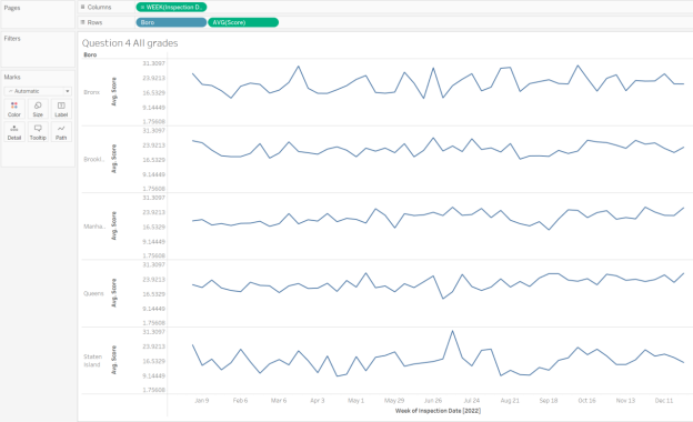
We can see that this is very sporadic data that doesn’t really show a clear pattern. Add “Grade” to the

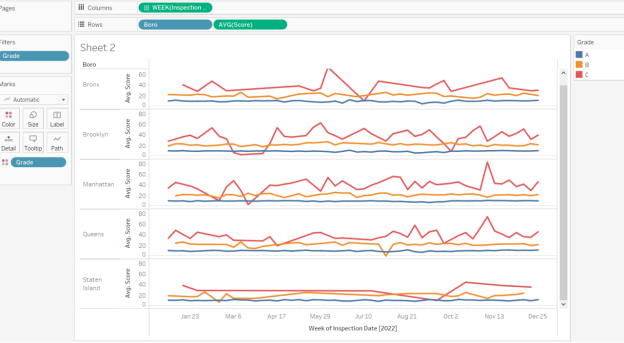
Question 4a: Based on these sparklines, which grade (A, B, or C) has a steady average score throughout the year for each borough (boro)?

A

B

C

Question 4A Answer:

A

Question 4b: Using the sparklines, which grade had the biggest average swings (increases and decreases) over the year?

A

B

C

Question 4B Answer:

C

Question 5: Dumbbell

In this exercise, you will look for crime patterns in the City of Baltimore that occur inside versus outside. To do this, we will use the dumbbell method. First, load the data source: September 2023 Baltimore City Crime Data: All Districts into Tableau, and start a new worksheet.

Drag the “All districts (Count)” measure into columns. Repeat this again (you will have two next to each other). Now drag “District” into the rows. Move “Inside Outside” into filters, and choose “Inside and Outside.”

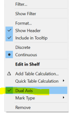
Right-click on the “CNT(All Districts)” column on the right, and select “Dual Axis.”

In the Marks area, change the first CNT(All Districts) to be a line. Drag “Inside Outside” onto the path marks area.

Make sure the second CNT(All Districts) mark is a circle. Now, drag “Inside Outside” onto the color inside that Marks menu.

You should have dumbbells that look like the following image:

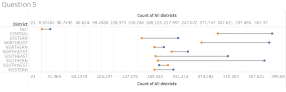
Question 5: Which district has a different pattern of inside crimes versus outside crimes compared to the other districts?

Option A: Central

Option B: Northeastern

Option C: Western

Option D: Southwestern

Question 5 Answer:

D: Southwestern

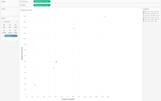
Question 6: Unit/symbol

We will be analyzing enrollment versus room capacity for a university. Load the dataset University courses and completion rates. Create a scatterplot by dragging “Student enrollment” and “Student Completed” onto columns and rows.

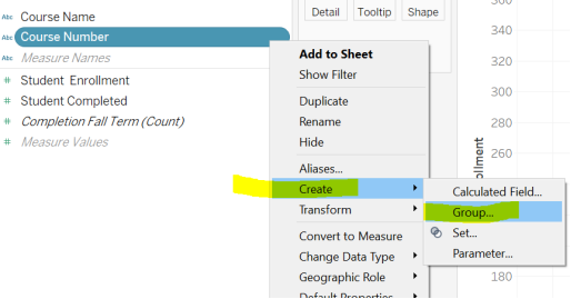
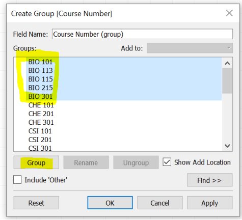
Now, we are going to make groups for each subject. Right-click on the “Course Number” dimension,  

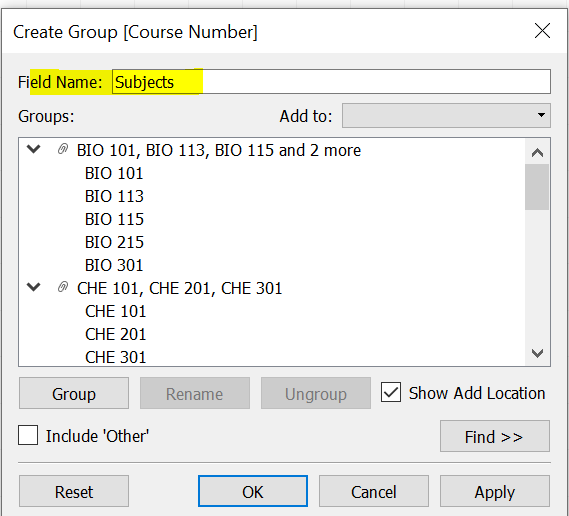
Now, drag that new field, “Subjects,” onto the “Shapes” mark.

We get a scatterplot that looks like this:

The problem is that our user has to look at the legend on the right to know what the subjects are. Let’s eliminate this problem by adding icons to make it easier for the user to read our graph.

Download the six icon image files that were provided to you in the assignment. You need to save them into your Tableau Repository file.

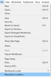
To find out where that file is, go under File ->Repository Location

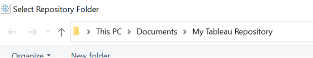
Make a note of the location where your Tableau Repository is located. In the image above, it is located in “Documents.” Go to the location of your Tableau Repository, and create a new folder called “University subjects.” Then copy and paste the six images provided to you into this folder.

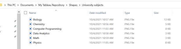
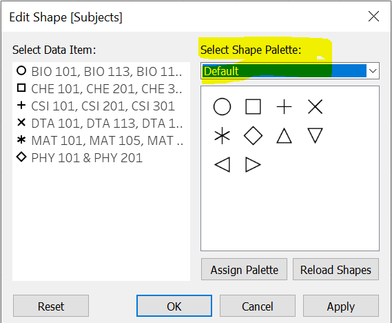
Change the Shape Palette from Default to University subjects. If you don’t see the shapes, click on “Reload Shapes.”
 

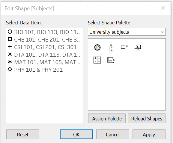
Now, you will assign the data item on the left to the appropriate icon on the right. They are both in alphabetical order.

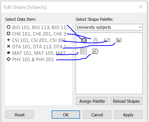
Click “Apply” when you are finished.

Your scatterplot probably has very small icons now:

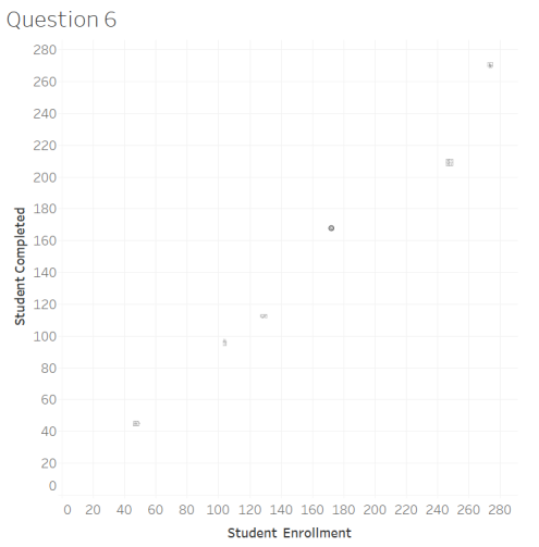
Question 6: Which subject has the lowest number of students enrolled and courses completed?

A: Math

B: Computer Science

C: Data Analytics

D: Physics

Question 6 Answer:

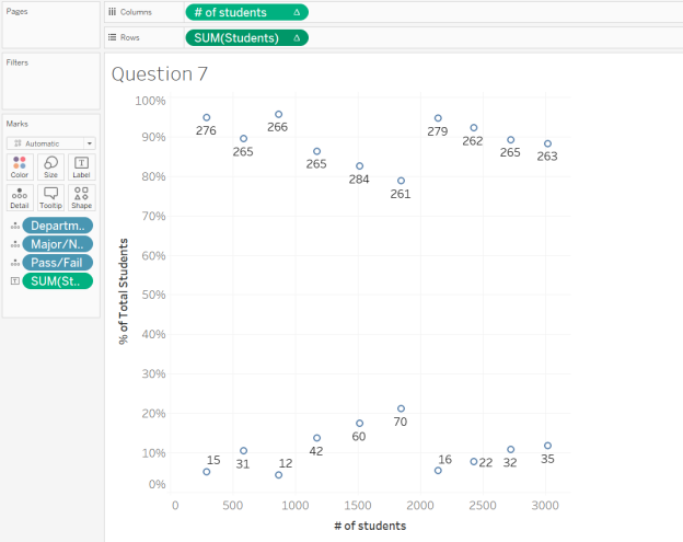
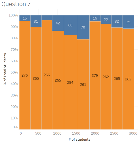
Question 7: Marimekko

The University we have been working with has asked for an analysis of the student pass/fail rates by major/nonmajor within six departments. Load the dataset: University pass rates.

Drag “Department,” “Major/NonMajor,” and “Pass/Fail” into rows. Drag “Students” onto the Label. You should see a simple table.

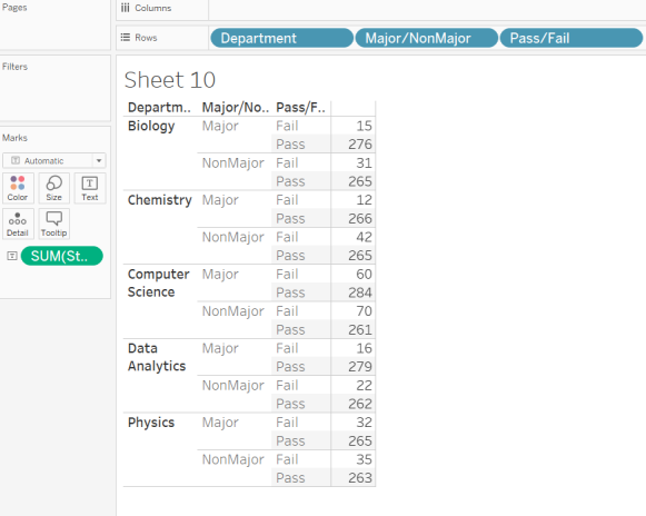
If we want to create a visualization across the three dimensions, we can create a Marimekko chart.

We need to create two calculated fields that will help us to get the right level of detail calculation for this analysis:

1. “Students per column” Syntax: {EXCLUDE [Pass/Fail]: SUM([Students])}
2. “# of students” Syntax:

IF FIRST()==0 THEN

MIN([Students per column])

ELSEIF MIN([Department]) != LOOKUP(MIN([Department]),-1) THEN

PREVIOUS_VALUE(0) + MIN([Students per column])

ELSEIF MIN([Major/NonMajor]) != LOOKUP(MIN([Major/NonMajor]),-1) THEN

PREVIOUS_VALUE(0) + MIN([Students per column])

ELSE

PREVIOUS_VALUE(0)

END

Move the three dimensions “Department,” “Major/NonMajor,” and “Pass/Fail” out of the rows and into the detail of the Marks area.

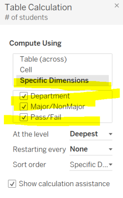
Drag the new calculated field: “# of students” into columns. Right-click to create a table calculation using across the dimensions “Department,” “Major/NonMajor,” and “Pass/Fail.”

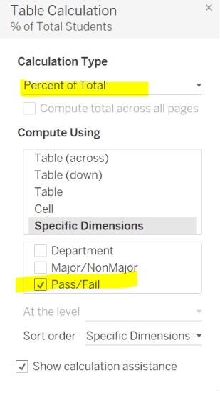
Drag the measure “Students” up into rows. Right-click, add table calculation: Percent of total, and compute using Pass/Fail.

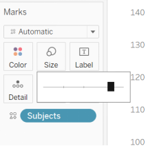
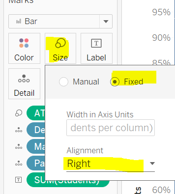
Drag “Students per column” into the size marks.

Click on the Size box, and change it to Fixed and Right alignment.

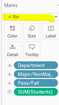
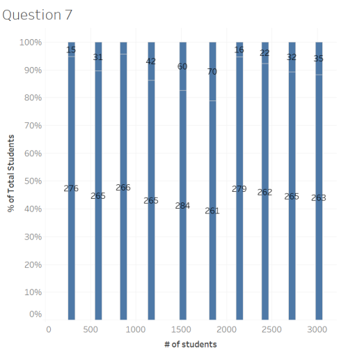
Drag “Pass/Fail” onto the Color mark. You should now have a bar chart like this:

Set a filter for “majors” only.

Add “Department” to the label.

Change the Label setting to “Allow labels to overlap.”

Question 7a: Which department had the most majors fail? (Hint: hover over the bars to look at the tooltips).

A: Biology

B: Chemistry

C: Computer Science

D: Data Analytics

E: Physics

Question 7a Answer:

Question 7b: What percentage of that department (from 7a) failed? (Hint: hover over the bars to look at the tooltips).

Question 7b Answer:

Question 8: Animated

For this animation, we will create a scatterplot using the Video game sales dataset. Create a new worksheet. Drag the measures “Global Sales” into columns and “Rank” into rows. Leave the aggregation as a SUM.

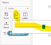
Drag “Platform” into Color. Change the Mark type to Circle. Click the size button to increase the size.

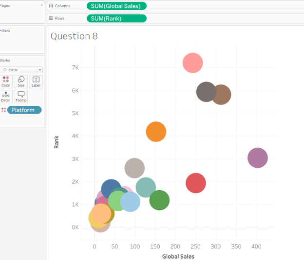
Drag “Genre” and “Platform” into the filters. Right-click, and select “Show filter” for each. Click “ok.” Make sure you have a blank scatterplot by ensuring no filters are selected.

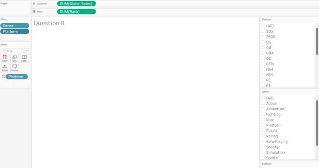
In your filters, click “PS” for the Platform and “Role-Playing” for Genre. Make a note of where the dot is located on the graph. What color is the dot?

Now, click “DS” for Platform; you should have two dots. Then click on “Puzzle” for Genre to add it as a filter.

Question 8: What happened to the PS dot? You can unclick the filters and apply them again to watch the animation.

Option A: Nothing changed

Option B: The PS dot dropped

Option C: The PS dot lifted

Option D: Both drops became equal

Question 8 Answer: