Task A – Data Acquisition and Exploratory Data Analysis
Data Acquisition
The dataset was obtained in Kaggle: Housing Price Prediction Dataset. It has 545 observations of houses, and the variables (price, area, bedrooms, parking) are numerical and categorical variables (furnishing status, access to main road, preferred area). Such a combination enables descriptive and inferential statistical analysis. The data can be used to comprehend the role of housing characteristics on the price of houses and it is relevant to real-life housing and urban planning decision-making.
Research Question
What are the structural and locational characteristics that the most severely affect house prices?
The statistical analysis and data visualization will be guided by this question with the main areas of concern: area, bedrooms, parking, main road access, furnishing status and preferred area.
Summary Statistics
The dataset contains 545 houses. The prices will be between 1.75 million and 13.3 million with the mean price of about 4.77 milliom (SD = 1.87 million). The size of houses ranges between 1,650 sq. ft and 16, 200 sq. ft with a median of 5,151 sq. ft. This implies that there is a good variety of housing stock with regard to affordability and property size.
| N | Minimum | Maximum | Mean | Std. Deviation | Variance | |
| Price of House | 545 | 1750000 | 13300000 | 4766729.25 | 1870439.616 | 3498544355820.582 |
| Area Coverage | 545 | 1650 | 16200 | 5150.54 | 2170.141 | 4709512.058 |
Frequency Distributions
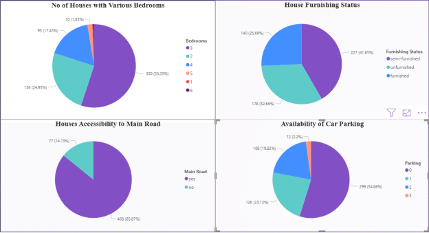
- Bedrooms: Most houses have 3 bedrooms (55%), followed by 2 bedrooms (24.95%), while larger homes (5–6 bedrooms) are rare (<3%).
- Main Road Access: A significant majority (85.87%) of properties are connected to the main road, highlighting accessibility as a common feature.
- Furnishing Status: The largest category is semi-furnished (41.65%), followed by furnished (25.69%) and unfurnished (32.66%).
- Parking: Over half the houses (54.86%) lack parking, 23.12% has a single parking lots, 19.82% has 2 parking slots and only 2.2% offer space for three vehicles.
TASK B – STATISTICAL ANALYSIS
Test 1: Correlation Analysis (Area vs. House Price)
- Hypotheses: There is a significant positive relationship between area and house price.
- Method: Pearson correlation (both variables are continuous).
- Assumptions: Linear relationship, normally distributed residuals.
Results:
| Correlations | |||
| Price of House | Area Coverage | ||
| Price of House | Pearson Correlation | 1 | .536** |
| Sig. (2-tailed) | .000 | ||
| N | 545 | 545 | |
| Area Coverage | Pearson Correlation | .536** | 1 |
| Sig. (2-tailed) | .000 | ||
| N | 545 | 545 | |
The Pearson correlation test was used to test the correlation between the house price and the area coverage. The findings were the existence of a moderate positive correlation (r = 0.536, p < 0.01) between the size of a house and its price, which means that the larger the house is, the more likely its price is to increase. This correlation is found to be significant and thus it is valid to state that big houses tend to fetch more money. This means that the hypothesis (H1) which states that area is a significant positive determinant of price is accepted.
Test 2: Independent Samples t-test (Main Road Access vs. House Price)
- Hypotheses: Houses with main road access have significantly different prices.
- Method: Independent t-test (group = main road access, dependent = price).
- Assumptions: Normality, homogeneity of variance.
Results:
T-Test
| Group Statistics | |||||
| Accesability to Main Road | N | Mean | Std. Deviation | Std. Error Mean | |
| Price of House | yes | 468 | 4991777.33 | 1893639.113 | 87533.499 |
| no | 77 | 3398904.55 | 894735.465 | 101964.569 | |
| Independent Samples Test | ||||||||||
| Levene’s Test for Equality of Variances | t-test for Equality of Means | |||||||||
| F | Sig. | t | df | Sig. (2-tailed) | Mean Difference | Std. Error Difference | 95% Confidence Interval of the Difference | |||
| Lower | Upper | |||||||||
| Price of House | Equal variances assumed | 30.624 | .000 | 7.245 | 543 | .000 | 1592872.784 | 219854.418 | 1161003.429 | 2024742.138 |
| Equal variances not assumed | 11.853 | 210.676 | .000 | 1592872.784 | 134383.358 | 1327964.463 | 1857781.105 | |||
| Independent Samples Effect Sizes | |||||
| Standardizera | Point Estimate | 95% Confidence Interval | |||
| Lower | Upper | ||||
| Price of House | Cohen’s d | 1787743.612 | .891 | .644 | 1.137 |
| Hedges’ correction | 1790217.618 | .890 | .643 | 1.136 | |
| Glass’s delta | 894735.465 | 1.780 | 1.406 | 2.149 | |
| a. The denominator used in estimating the effect sizes. Cohen’s d uses the pooled standard deviation. Hedges’ correction uses the pooled standard deviation, plus a correction factor. Glass’s delta uses the sample standard deviation of the control group. | |||||
The independent t-test was used to compare the prices of houses depending on the access to the main road. An average price of houses with access to the roads (4,991,777.33) was higher than the unaccessible ones (3,398,904.55). The gap between the two figures amounted to 1,592,872.78 which was also statistically insignificant (t = 7.245, p < 0.01) and the effect size was quite large (Cohen d = 0.891). This demonstrates that accessibility has a strong effect on price. Therefore, the null hypothesis (H2) is accepted: houses which have access to the main road are much more expensive.
Test 3: One-Way ANOVA (Furnishing Status vs. House Price)
- Hypotheses: furnishing category has a significantly different mean price.
- Method: One-Way ANOVA (independent = furnishing status, dependent = price).
- Assumptions: Normality, homogeneity of variance.
Results:
Oneway
| Descriptives | ||||||||
| Price of Houses | ||||||||
| N | Mean | Std. Deviation | Std. Error | 95% Confidence Interval for Mean | Minimum | Maximum | ||
| Lower Bound | Upper Bound | |||||||
| furnished | 141 | 5496435.74 | 2110297.458 | 177719.106 | 5145075.53 | 5847795.96 | 1750000 | 13300000 |
| semi-furnished | 227 | 4907524.23 | 1596687.757 | 105975.889 | 4698697.02 | 5116351.44 | 1767150 | 12250000 |
| unfurnished | 177 | 4004870.06 | 1720955.307 | 129354.922 | 3749583.67 | 4260156.44 | 1750000 | 10150000 |
| Total | 545 | 4766729.25 | 1870439.616 | 80120.830 | 4609345.15 | 4924113.35 | 1750000 | 13300000 |
| Tests of Homogeneity of Variances | |||||
| Levene Statistic | df1 | df2 | Sig. | ||
| Price of Houses | Based on Mean | 8.337 | 2 | 542 | .000 |
| Based on Median | 7.288 | 2 | 542 | .001 | |
| Based on Median and with adjusted df | 7.288 | 2 | 530.937 | .001 | |
| Based on trimmed mean | 8.121 | 2 | 542 | .000 | |
| ANOVA | |||||
| Price of Houses | |||||
| Sum of Squares | df | Mean Square | F | Sig. | |
| Between Groups | 182314372711905.120 | 2 | 91157186355952.560 | 28.710 | .000 |
| Within Groups | 1720893756854486.000 | 542 | 3175080732203.849 | ||
| Total | 1903208129566391.000 | 544 | |||
Post Hoc Tests
| Multiple Comparisons | ||||||
| Dependent Variable: Price of Houses | ||||||
| Tukey HSD | ||||||
| (I) furnishingstatus | (J) furnishingstatus | Mean Difference (I-J) | Std. Error | Sig. | 95% Confidence Interval | |
| Lower Bound | Upper Bound | |||||
| furnished | semi-furnished | 588911.516* | 191063.976 | .006 | 139879.15 | 1037943.88 |
| unfurnished | 1491565.688* | 201138.291 | .000 | 1018857.00 | 1964274.38 | |
| semi-furnished | furnished | -588911.516* | 191063.976 | .006 | -1037943.88 | -139879.15 |
| unfurnished | 902654.173* | 178676.940 | .000 | 482733.42 | 1322574.93 | |
| unfurnished | furnished | -1491565.688* | 201138.291 | .000 | -1964274.38 | -1018857.00 |
| semi-furnished | -902654.173* | 178676.940 | .000 | -1322574.93 | -482733.42 | |
| *. The mean difference is significant at the 0.05 level. | ||||||
Homogeneous Subsets
| Price of Houses | ||||
| Tukey HSDa,b | ||||
| furnishingstatus | N | Subset for alpha = 0.05 | ||
| 1 | 2 | 3 | ||
| unfurnished | 177 | 4004870.06 | ||
| semi-furnished | 227 | 4907524.23 | ||
| furnished | 141 | 5496435.74 | ||
| Sig. | 1.000 | 1.000 | 1.000 | |
| Means for groups in homogeneous subsets are displayed. | ||||
| a. Uses Harmonic Mean Sample Size = 174.956. | ||||
| b. The group sizes are unequal. The harmonic mean of the group sizes is used. Type I error levels are not guaranteed. | ||||
The ANOVA used was a one-way test, which studied the differences in prices of houses in various categories of furnishing. The findings showed a big difference in the mean prices (F (2, 542) = 28.71, p = 0.01). The average price of furnished houses was the highest (5,496,435.74), semi-furnished (4,907,524.23) and unfurnished houses came next (4,004,870.06). Post-hoc Tukey tests were done to ensure that the three groups are significantly different (p < 0.05). This was a significant impact, which demonstrated that the status of furnishing has a significant impact on property value. Thus, hypothesis (H3) is accepted: furnishing categories differ in terms of house prices significantly.
Interpretation Across Tests
The three statistical tests together highlight the key drivers of house price variation in the dataset.
- Correlation (Area vs. Price): The Pearson correlation showed a moderate positive relationship (r = 0.536, p < 0.01), meaning larger houses tend to have higher prices. This indicates that area coverage is a strong structural factor in determining property value.
- T-test (Main Road Access vs. Price): Results revealed a significant difference in mean prices between houses with road access (M = 4.9M) and those without (M = 4.0M), with a large effect size (Cohen’s d ≈ 0.89). This suggests that location and accessibility are crucial in price determination, as buyers are willing to pay more for well-connected properties.
- ANOVA (Furnishing Status vs. Price): The ANOVA confirmed that furnishing levels significantly impact house prices. Furnished houses had the highest mean price (≈ 5.5M), followed by semi-furnished (≈ 4.9M) and unfurnished (≈ 4.0M). Post-hoc comparisons showed that all groups differ significantly (p < 0.05). This underlines how value-added amenities and presentation enhance property worth.
DATA VISUALIZATIONS
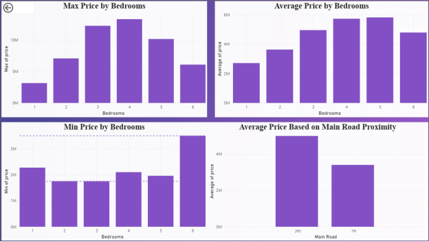
- Max Price by Bedrooms: Shows the highest house prices observed for each bedroom count. Houses with 4 bedrooms recorded the highest maximum prices.
- Average Price by Bedrooms: Illustrates how mean prices rise with additional bedrooms, peaking around 4–5 bedrooms.
- Min Price by Bedrooms: Highlights the lowest prices in each bedroom category. Interestingly, 6-bedroom houses show higher minimum prices compared to smaller houses.
- Average Price Based on Main Road Proximity: Demonstrates that houses with main road access have higher average prices than those without.
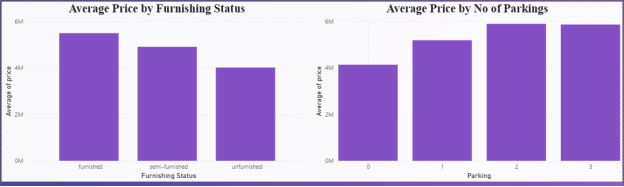
- Average Price by Furnishing Status: Furnished houses have the highest average prices, followed by semi-furnished, with unfurnished being the lowest.
- Average Price by Number of Parkings: Indicates that more parking spaces are linked to higher house prices, with 2–3 parking slots showing the highest averages.
CONCLUSION
This research examined the determinants of the prices of houses through three statistical methods and the findings of the study combinedly indicate the combined effect of size, location, and furnishing to the determination of the house prices. Firstly, correlation analysis has depicted a moderate positive correlation between the area coverage and the price; thus, it has been proved that bigger houses tend to be priced higher. Second, the independent t-test supported the hypothesis that houses with main road access cost considerably more than houses without access to it, which serves to highlight the value of the location and its accessibility as a factor that buyers consider when purchasing a house. Lastly, the one-way ANOVA showed a great difference in prices of the categories of furnished things and the highest price was that of furnished homes, then semi furnished, and then the unfurnished. The combined results confirm all the three assumptions, as they prove that the trend in the housing market is the result of the interaction of the structural features, the accessibility of the context, and the quality of furnishings. This information is useful to homeowners, investors and policymakers who would like to maximize the value of their property and make decisions that help them to make informed choices on the housing market.