Introduction:
Cost and management accounting is the process of ascertaining product and service related cost information in detailed and analysis of such information which can help in making various important business decisions such as make or buy decision, shut down decision and so on. In this report, some of such cost and management tools and techniques have been applied and analyzed with the help of some real life information of the Motomart as given in the case study. In the first part the five years income statement has been reviewed and analyzed and in the second part, the behavior of expenses and its level of activities have been discussed. The cost equation has been formulated using the excel spreadsheet model for projection and analysis of cost structure and lastly, the findings have been summarized for recapitulation of the whole analysis (Collis & Hussey 2017).
Step 1: Analysis of the 5 Years Income Statement:
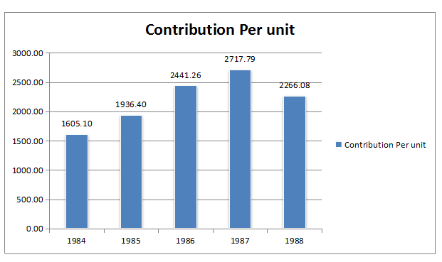
In the case study, the income statement of Motomart has been given for the year 1984 to 1988. They have given some measures of the income statement and some exhibit of the income statement, which will help us in analyzing the financial performance and financial position of the Motomart. It can be observed from the given five year income statement that, the sale volume is having a fluctuation and it was highest in the year 1998 and the lowest sales volume was marked in the year 1987. The contribution margin per unit is calculated as the difference between the sales price per unit and the variable cost per unit. It can be observed from the given information that, the contribution margin per unit in the year 1984 was $1,605.10 and it becomes the highest in the year 1987 for an amount of $2,717.79, thereafter it comes to $2,26.08 in the year 1988. It can be commented in this context that, in the initial years the company was able to manage their operating activities and was efficient enough to reduce the variable cost by eliminating the wastage. They achieved the highest efficiency in the year 1887. It can be presented with the help of the following chart.
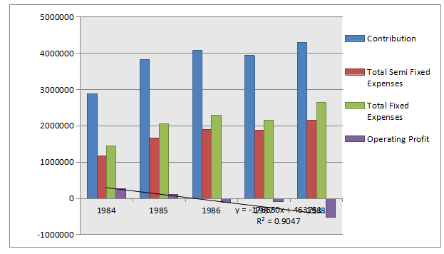
It can be noticed from their income statement that, there is a decreasing trend in their profitability and they have incurred a huge loss in the year 1989. There are several reasons for such a loss and the increased fixed cost burden might be one most important of them. It can be observed that, the total fixed cost has been increased over the years and it became $2,653,620 in the year 1989 while it was only $1,449,208 in the year 1984. There is an increase of $1,204,412 over the five years. On the other hand the variable cost expenses per unit have been increased in the year 1989 as compared to the preceding year 1988. Therefore, it can be commented that, the huge amount of loss in the year 1989 was due to the increased fixed cost and variable costs. There was a decrease in the volume of sales in the year 1986 and 1987. As the total fixed costs was having an increasing trend the decrease in number of unit sales results in higher allocation of fixed costs per unit and in turn results into a loss. There is also an abnormal trend and fluctuation in the total semi fixed costs. With the decrease in number of sales in the year 1986 the semi fixed costs should have been decreased also. But the same trend was not followed in the income statement of the Motomart. It implies that the fixed part of the semi fixed costs expenses was also following an increasing trend. The overall components of the expenses and income can be shown with the help of the following bar chart.
From the above analysis, it can be commented that, the company needs to concentrate on managing its fixed expenses and they need to set such units of output which will give them the economies of scale. They need to ensure the optimum utilization of the resources and facilities. If the production volume can be set to the optimum level which will make the distribution of fixed costs thinly to the production units, they can make a significant amount of profit. As they are able to manage their variable costs which is depicted by their increasing contribution margin per unit, efficient management of fixed costs might give them a better solution.
Step 2: Pattern in expenses item:
In the five year income statement the net sales revenues have been given as the sales revenue less variable costs. And it can be observed that there is a gradual decrease in the variable costs per unit as the contribution per unit is increasing. There are eight components in the total semi fixed costs. It can be observed that the salary expenses are having an annual hike which might because of increase in the salary structure every year. Vacation costs is having some abnormalities and do not follow any fixed pattern. It depends on certain situations and if such situation arises then the costs are incurred. It can be observed that in the first year there was the lowest amount of vacation costs. The advertisement costs are a period costs and follows almost the same pattern over the year with a marginal increasing trend. Rests of the components of the semi fixed costs are variable in nature but there are some negative figures in the schedule of costs can be observed. Costs can be zero but it should not be negative by no means unless there is any revenue arising from such components. Hence, it can be commented that, the semi fixed costs can again be bifurcated into fixed and variable parts. Salary and advertisement costs depends on the time period and remaining parts of the semi fixed costs are mainly variable in nature, but it do not follow an unitary relationship with the volume of output.
Step 3: High Low Activity Level:
High low method is a tool used in cost accounting to separate the fixed and variable parts of the semi fixed costs. In the given case study of Motomart, to separate the semi fixed costs the same technique can be applied (Collis & Hussey 2017). To do that the high and low measures of each of the cost components can be identified as in the following table.
| Expenses | High | Low |
| Salaries | 1,28,007 | 45,491 |
| Vacation | 9,212 | – |
| Advertising and Training | 38,616 | 9,112 |
| Supplies/Tools/Laundry | 14,426 | -684 |
| Freight | 1,628 | -492 |
| Vehicle | 3,175 | 486 |
| Demonstrator | 4,517 | -3,513 |
| Floor-Planning | 1,88,040 | -78,173 |
The high measures of expenses are identified from the given cost statement but it is not matching with the activity level. In most of the cases the high and low expenses are not coming in the NVRS 280 and 31.
Step 4: Computation of Cost Equations:
Using the cost equation and the high low technique the semi fixed costs can be separated into variable costs per unit and fixed costs as given in the following table.
| Expenses | FC | VC | R-sq |
| Salaries | 1,06,866 | -110 | 4.07% |
| Vacation | 1,194 | 1 | 0.17% |
| Advertising and Training | 24,348 | -0 | 0.00% |
| Supplies/Tools/Laundry | 8,269 | -22 | 9.28% |
| Freight | 430 | 0 | 0.17% |
| Vehicle | 1,809 | 0 | 0.03% |
| Demonstrator | 1,305 | -7 | 3.85% |
| Floor-Planning | 80,537 | -400 | 28.32% |
| Computed Total | 2,24,758 | -537 | 24.67% |
| Total | 4,49,517 | -1,074 | 70.56% |
Answer to question 1:
There are some errors in the data provided that is why the computed R-square in case of advertisement and vehicles expenses are coming to a zero. There is no parity with the activity level and the expenses.
Answer to question 2:
The R-square is the measure of goodness of fit and the total R-square is 70.56% which indicates a high goodness of fit. It implies the result is depicting the seventy percent variability of the data.
Answer to question 3:
Slopes are negative for most of the expenses and it is positive only for the vacation costs. The total slope is negative.
Answer to question 4:
The results are not consistent with the high low calculation of the fixed and variable costs. There is a huge difference between these two computations.
Step 5: Findings from the analysis:
From the above discussion and analysis, it can be concluded that, the data for the Motomart as has been given in the case study are full of errors. There is no parity with the expenses and the respective activity levels; hence, it cannot be used for financial forecasting reliably. If customers need to use these forecasts as has been prepared based on the given data, the they should be concentrating on the behavior of costs more carefully as the data provided by the Motomart do not completely exhibit the exact behavior and their pattern. Therefore, these forecasts are not reliable and needs correction for a reliable and realistic projection of the expenses.
References and bibliography:
Collis, J., & Hussey, R. (2017). Cost and management accounting. Macmillan International Higher Education.
Cooper, R. (2017). Supply chain development for the lean enterprise: interorganizational cost management. Routledge.
Fullerton, R. R., Kennedy, F. A., & Widener, S. K. (2014). Lean manufacturing and firm performance: The incremental contribution of lean management accounting practices. Journal of Operations Management, 32(7-8), 414-428.
Kaplan, R. S., & Atkinson, A. A. (2015). Advanced management accounting. PHI Learning.
Klychova, G. S., Faskhutdinova, М. S., & Sadrieva, E. R. (2014). Budget efficiency for cost control purposes in management accounting system. Mediterranean journal of social sciences, 5(24), 79.
Kokubu, K., & Kitada, H. (2015). Material flow cost accounting and existing management perspectives. Journal of Cleaner Production, 108, 1279-1288.
Maskell, B. H., Baggaley, B., & Grasso, L. (2017). Practical lean accounting: a proven system for measuring and managing the lean enterprise. Productivity Press.